cartesian_uniform_1d
Uniform 1-D Cartesian grid with consumer-supplied extent: N cell-centered points, cell centers x_i = x0 + (i - 1/2) dx. The index set x is the iteration axis; N (the cell count) remains the esm-spec 9.7 metaparameter, bound at the import edge or the loader API. The real-valued geometry is NOT baked into this file: x0 (left domain edge) and dx (cell spacing) are free names in the x_coord template body (and in this grid’s stencils/rules), resolving in the consuming component’s scope at evaluation — the same keyed-factor contract grids/mpas uses for areaCell/dvEdge. A consuming model MUST define both as ordinary real-valued model variables: for a domain [a, b], x0 = a (parameter, default a) and dx = (b - a)/N (an observed variable whose expression divides the extent by the metaparameter name N, e.g. {op: /, args: [b - a, N]}, so that a loader-API rebinding of N — a convergence sweep — keeps dx consistent automatically; spec 9.7.6 substitutes the document-scoped N as an integer literal in expression positions at load). A model that binds N at the import edge closes N before it reaches the model’s own scope, and must instead spell dx with the matching literal (e.g. {op: /, args: [1, 8]} for N=8 on the unit interval).
Metaparameters
| Name | Type | Default | Description |
|---|---|---|---|
N | integer | 64 | Number of cells along x. |
All sizes are load-time metaparameters (esm-spec §9.7.6): rebind them at the import edge (or through the loader API) and the same files serve every resolution.
Consumer-supplied free names
The geometry is consumer-supplied so the same files serve any domain extent, not just any resolution. For a domain [a, b] the consuming model defines x0 = a (a parameter) and dx = (b − a)/N (an observed whose expression divides by the metaparameter name N, so a loader-API rebinding of N — a convergence sweep — keeps dx consistent). A model that instead closes N at the import edge spells the matching literal ({op: /, args: [1, 8]} for N = 8 on the unit interval). See the extent proof problems/heat_1d_zero_grad_nonunit.esm (x ∈ [−1.5, 2.5], observed order 2.00).
Index sets
| Name | Kind | Size |
|---|---|---|
x | interval | N |
Geometry templates
| Template | Definition | Description |
|---|---|---|
x_coord | x_coord[i] = x0 + (i − 0.5)·dx for i ∈ x | Cell-center coordinates x_i = x0 + (i - 1/2) dx, shaped over the x index set. x0 and dx are free names supplied by the consuming model (see metadata.description for the contract). |
Stencils
Interior-only, match-less templates importing grid.esm; the rules below wrap them with boundary-condition face regions into complete rewrite rules.
central_D1_interior
Source: grids/cartesian_uniform_1d/stencils/central_D1_interior.esm
Interior-only 3-point centered first derivative on cartesian_uniform_1d: (f[i+1] - f[i-1]) / (2 dx) over i in [2, N-1]. Match-less named template; boundary-condition layers (rules/) wrap it into complete rewrite rules. dx is a free name resolving to the consuming model’s spacing variable (the grid’s consumer-supplied geometry contract; see grids/cartesian_uniform_1d/grid.esm). O(dx^2) on this uniform grid.
References
- Fornberg, B. (1988). Generation of finite difference formulas on arbitrarily spaced grids. Mathematics of Computation 51(184), 699-706.
doi:10.1090/S0025-5718-1988-0935077-0
central_D2_4_dirichlet_face1
Source: grids/cartesian_uniform_1d/stencils/central_D2_4_dirichlet_face1.esm
Fourth-order one-sided second-derivative closure for the cell nearest a Dirichlet (fixed-value) wall on cartesian_uniform_1d, cell-centered. Match-less named scalar template; the boundary-condition rule (rules/central_D2_4_dirichlet_bc) applies it at the first interior row against a prescribed wall value. On this cell-centered grid the wall sits half a cell outside the first center, so the wall value g and the five nearest cell values sit at offsets {0, 1/2, 3/2, 5/2, 7/2, 9/2}*dx from the wall. The unique degree-5 polynomial through those six data, differentiated twice at the first center (offset 1/2 dx), gives D2 = (2560 g - 4095 f1 + 1848 f2 - 378 f3 + 72 f4 - 7 f5) / (756 dx^2), where f1..f5 are the five cells in order of increasing distance from the wall and g is the wall value (Fornberg 1988 weights for the offset node set). Because six data fit a quintic, the second derivative is exact for polynomials up to degree 5 and the local truncation error is O(dx^4) — matching the interior 5-point stencil central_D2_4_interior, so the global scheme stays fourth order with no boundary reduction. A linear (degree-1) field is reproduced exactly and returns identically zero (the sum of all six weights is zero), so a steady linear profile carrying the wall value is discretely exact. Reused unchanged at the right wall by reflection (the second derivative is even under x -> -x), with f1..f5 mapped to the cells in increasing distance from the right wall and g bound to the right wall value. dx is a free name resolving to the consuming model’s spacing variable (the grid’s consumer-supplied geometry contract; see grids/cartesian_uniform_1d/grid.esm).
References
- Fornberg, B. (1988). Generation of finite difference formulas on arbitrarily spaced grids. Mathematics of Computation 51(184), 699-706.
doi:10.1090/S0025-5718-1988-0935077-0
central_D2_4_dirichlet_face2
Source: grids/cartesian_uniform_1d/stencils/central_D2_4_dirichlet_face2.esm
Fourth-order one-sided second-derivative closure for the SECOND cell from a Dirichlet (fixed-value) wall on cartesian_uniform_1d, cell-centered. Match-less named scalar template; the boundary-condition rule (rules/central_D2_4_dirichlet_bc) applies it at the second interior row, whose centered 5-point stencil would reach one cell outside the domain. The same six data as central_D2_4_dirichlet_face1 (the wall value g at offset 0 and the five nearest cells f1..f5 at offsets {1/2,3/2,5/2,7/2,9/2}*dx) fit a degree-5 polynomial; differentiating it twice at the SECOND center (offset 3/2 dx) gives D2 = (-256 g + 1323 f1 - 2100 f2 + 1134 f3 - 108 f4 + 7 f5) / (756 dx^2) (Fornberg 1988 weights for the offset node set and this evaluation point). Exact for polynomials up to degree 5, so the local truncation error is O(dx^4), matching the interior 5-point stencil; the six weights sum to zero, so a steady linear profile is discretely exact and returns identically zero. Reused unchanged at the right wall’s second cell by reflection (the second derivative is even under x -> -x), with f1..f5 mapped to the cells in increasing distance from the right wall and g bound to the right wall value. dx is a free name resolving to the consuming model’s spacing variable (the grid’s consumer-supplied geometry contract; see grids/cartesian_uniform_1d/grid.esm).
References
- Fornberg, B. (1988). Generation of finite difference formulas on arbitrarily spaced grids. Mathematics of Computation 51(184), 699-706.
doi:10.1090/S0025-5718-1988-0935077-0
central_D2_4_interior
Source: grids/cartesian_uniform_1d/stencils/central_D2_4_interior.esm
Interior-only 5-point fourth-order centered second derivative on cartesian_uniform_1d: (-f[i-2] + 16 f[i-1] - 30 f[i] + 16 f[i+1] - f[i+2]) / (12 dx^2) over i in [3, N-2]. Match-less named template; boundary-condition layers (rules/) wrap it into complete rewrite rules. dx is a free name resolving to the consuming model’s spacing variable (the grid’s consumer-supplied geometry contract; see grids/cartesian_uniform_1d/grid.esm). O(dx^4) on this uniform grid — the 4th-order companion to the 3-point central_D2_interior.
References
- Fornberg, B. (1988). Generation of finite difference formulas on arbitrarily spaced grids. Mathematics of Computation 51(184), 699-706.
doi:10.1090/S0025-5718-1988-0935077-0
central_D2_4_neumann_face1
Source: grids/cartesian_uniform_1d/stencils/central_D2_4_neumann_face1.esm
Fourth-order one-sided second-derivative closure for the cell nearest a Neumann (fixed-flux) wall on cartesian_uniform_1d, cell-centered. Match-less named scalar template; the boundary-condition rule (rules/central_D2_4_neumann_bc) applies it at the first interior row against a prescribed wall gradient. The datum is the wall derivative q = du/dx at the wall (offset 0) together with the five nearest cell values f1..f5 at offsets {1/2,3/2,5/2,7/2,9/2}*dx. The unique degree-5 Hermite-type polynomial matching those six data (one derivative datum + five values) differentiated twice at the first center (offset 1/2 dx) gives D2 = (-19200 q dx - 15285 f1 + 7544 f2 + 12546 f3 - 5784 f4 + 979 f5) / (20268 dx^2) (Fornberg 1988 weights for the offset node set with a derivative constraint at the wall). Six data fit a quintic, so the second derivative is exact for polynomials up to degree 5 and the local truncation error is O(dx^4) — matching the interior 5-point stencil central_D2_4_interior, so the global scheme stays fourth order. A linear (degree-1) field is reproduced exactly: the five value-weights sum to zero and the derivative term supplies the exact wall slope, so a steady ramp with the matching wall flux returns identically zero and is discretely exact. The template is written for a LEFT (low-index) wall where q = +du/dx points into the domain. It is reused unchanged at the right wall by reflection (the second derivative is even under x -> -x, but du/dx is odd), so the rule binds q -> -qR there (the derivative datum negates under reflection) with f1..f5 mapped to the cells in increasing distance from the right wall. dx is a free name resolving to the consuming model’s spacing variable (the grid’s consumer-supplied geometry contract; see grids/cartesian_uniform_1d/grid.esm).
References
- Fornberg, B. (1988). Generation of finite difference formulas on arbitrarily spaced grids. Mathematics of Computation 51(184), 699-706.
doi:10.1090/S0025-5718-1988-0935077-0
central_D2_4_neumann_face2
Source: grids/cartesian_uniform_1d/stencils/central_D2_4_neumann_face2.esm
Fourth-order one-sided second-derivative closure for the SECOND cell from a Neumann (fixed-flux) wall on cartesian_uniform_1d, cell-centered. Match-less named scalar template; the boundary-condition rule (rules/central_D2_4_neumann_bc) applies it at the second interior row, whose centered 5-point stencil would reach one cell outside the domain. The same six data as central_D2_4_neumann_face1 (the wall derivative q = du/dx at offset 0 and the five nearest cells f1..f5 at offsets {1/2,3/2,5/2,7/2,9/2}*dx) determine the degree-5 Hermite-type polynomial; differentiating it twice at the SECOND center (offset 3/2 dx) gives D2 = (1920 q dx + 26019 f1 - 52100 f2 + 28134 f3 - 2124 f4 + 71 f5) / (20268 dx^2) (Fornberg 1988 weights for the offset node set with a derivative constraint at the wall). Exact for polynomials up to degree 5, so the local truncation error is O(dx^4), matching the interior 5-point stencil; the five value-weights sum to zero and the derivative term supplies the exact wall slope, so a steady ramp with the matching wall flux is discretely exact. Written for a LEFT (low-index) wall where q = +du/dx points into the domain; reused unchanged at the right wall’s second cell by reflection (the second derivative is even, du/dx odd), so the rule binds q -> -qR there with f1..f5 mapped to the cells in increasing distance from the right wall. dx is a free name resolving to the consuming model’s spacing variable (the grid’s consumer-supplied geometry contract; see grids/cartesian_uniform_1d/grid.esm).
References
- Fornberg, B. (1988). Generation of finite difference formulas on arbitrarily spaced grids. Mathematics of Computation 51(184), 699-706.
doi:10.1090/S0025-5718-1988-0935077-0
central_D2_6_dirichlet_face1
Source: grids/cartesian_uniform_1d/stencils/central_D2_6_dirichlet_face1.esm
Sixth-order one-sided second-derivative closure for the cell nearest a Dirichlet (fixed-value) wall on cartesian_uniform_1d, cell-centered. Match-less named scalar template; the boundary-condition rule (rules/central_D2_6_dirichlet_bc) applies it at the first interior row against a prescribed wall value. On this cell-centered grid the wall sits half a cell outside the first center, so the wall value g and the seven nearest cell values sit at offsets {0, 1/2, 3/2, 5/2, 7/2, 9/2, 11/2, 13/2}*dx from the wall. The unique degree-7 polynomial through those eight data, differentiated twice at the first center (offset 1/2 dx), gives D2 = (86016 g - 136136 f1 + 56628 f2 - 3861 f3 - 5720 f4 + 4290 f5 - 1404 f6 + 187 f7) / (25740 dx^2), where f1..f7 are the seven cells in order of increasing distance from the wall and g is the wall value (Fornberg 1988 weights for the offset node set). Because eight data fit a septic, the second derivative is exact for polynomials up to degree 7 and the local truncation error is O(dx^6) — matching the interior 7-point stencil central_D2_6_interior, so the interior order is preserved at the wall. A linear (degree-1) field is reproduced exactly and returns identically zero (the sum of all eight weights is zero: 86016 - 136136 + 56628 - 3861 - 5720 + 4290 - 1404 + 187 = 0), so a steady linear profile carrying the wall value is discretely exact. Reused unchanged at the right wall by reflection (the second derivative is even under x -> -x), with f1..f7 mapped to the cells in increasing distance from the right wall and g bound to the right wall value. dx is a free name resolving to the consuming model’s spacing variable (the grid’s consumer-supplied geometry contract; see grids/cartesian_uniform_1d/grid.esm).
References
- Fornberg, B. (1988). Generation of finite difference formulas on arbitrarily spaced grids. Mathematics of Computation 51(184), 699-706.
doi:10.1090/S0025-5718-1988-0935077-0
central_D2_6_dirichlet_face2
Source: grids/cartesian_uniform_1d/stencils/central_D2_6_dirichlet_face2.esm
Sixth-order one-sided second-derivative closure for the SECOND cell from a Dirichlet (fixed-value) wall on cartesian_uniform_1d, cell-centered. Match-less named scalar template; the boundary-condition rule (rules/central_D2_6_dirichlet_bc) applies it at the second interior row, whose centered 7-point stencil would reach two cells outside the domain. The same eight data as central_D2_6_dirichlet_face1 (the wall value g at offset 0 and the seven nearest cells f1..f7 at offsets {1/2,3/2,5/2,7/2,9/2,11/2,13/2}*dx) fit a degree-7 polynomial; differentiating it twice at the SECOND center (offset 3/2 dx) gives D2 = (-2048 g + 11349 f1 - 17745 f2 + 8073 f3 + 1170 f4 - 1105 f5 + 351 f6 - 45 f7) / (7020 dx^2) (Fornberg 1988 weights for the offset node set and this evaluation point). Exact for polynomials up to degree 7, so the local truncation error is O(dx^6), matching the interior 7-point stencil; the eight weights sum to zero (-2048 + 11349 - 17745 + 8073 + 1170 - 1105 + 351 - 45 = 0), so a steady linear profile is discretely exact and returns identically zero. Reused unchanged at the right wall’s second cell by reflection (the second derivative is even under x -> -x), with f1..f7 mapped to the cells in increasing distance from the right wall and g bound to the right wall value. dx is a free name resolving to the consuming model’s spacing variable (the grid’s consumer-supplied geometry contract; see grids/cartesian_uniform_1d/grid.esm).
References
- Fornberg, B. (1988). Generation of finite difference formulas on arbitrarily spaced grids. Mathematics of Computation 51(184), 699-706.
doi:10.1090/S0025-5718-1988-0935077-0
central_D2_6_dirichlet_face3
Source: grids/cartesian_uniform_1d/stencils/central_D2_6_dirichlet_face3.esm
Sixth-order one-sided second-derivative closure for the THIRD cell from a Dirichlet (fixed-value) wall on cartesian_uniform_1d, cell-centered. Match-less named scalar template; the boundary-condition rule (rules/central_D2_6_dirichlet_bc) applies it at the third interior row, whose centered 7-point stencil would reach one cell outside the domain. The same eight data as central_D2_6_dirichlet_face1/face2 (the wall value g at offset 0 and the seven nearest cells f1..f7 at offsets {1/2,3/2,5/2,7/2,9/2,11/2,13/2}*dx) fit a degree-7 polynomial; differentiating it twice at the THIRD center (offset 5/2 dx) gives D2 = (4096 g - 17589 f1 + 121836 f2 - 216216 f3 + 120120 f4 - 13585 f5 + 1404 f6 - 66 f7) / (77220 dx^2) (Fornberg 1988 weights for the offset node set and this evaluation point). Exact for polynomials up to degree 7, so the local truncation error is O(dx^6), matching the interior 7-point stencil; the eight weights sum to zero (4096 - 17589 + 121836 - 216216 + 120120 - 13585 + 1404 - 66 = 0), so a steady linear profile is discretely exact and returns identically zero. Reused unchanged at the right wall’s third cell by reflection (the second derivative is even under x -> -x), with f1..f7 mapped to the cells in increasing distance from the right wall and g bound to the right wall value. dx is a free name resolving to the consuming model’s spacing variable (the grid’s consumer-supplied geometry contract; see grids/cartesian_uniform_1d/grid.esm).
References
- Fornberg, B. (1988). Generation of finite difference formulas on arbitrarily spaced grids. Mathematics of Computation 51(184), 699-706.
doi:10.1090/S0025-5718-1988-0935077-0
central_D2_6_interior
Source: grids/cartesian_uniform_1d/stencils/central_D2_6_interior.esm
Interior-only 7-point sixth-order centered second derivative on cartesian_uniform_1d: (2 f[i-3] - 27 f[i-2] + 270 f[i-1] - 490 f[i] + 270 f[i+1] - 27 f[i+2] + 2 f[i+3]) / (180 dx^2) over i in [4, N-3]. Match-less named template; boundary-condition layers (rules/) wrap it into complete rewrite rules. dx is a free name resolving to the consuming model’s spacing variable (the grid’s consumer-supplied geometry contract; see grids/cartesian_uniform_1d/grid.esm). O(dx^6) on this uniform grid — the 6th-order member of the central_D2 family.
References
- Fornberg, B. (1988). Generation of finite difference formulas on arbitrarily spaced grids. Mathematics of Computation 51(184), 699-706.
doi:10.1090/S0025-5718-1988-0935077-0
central_D2_6_neumann_face1
Source: grids/cartesian_uniform_1d/stencils/central_D2_6_neumann_face1.esm
Sixth-order one-sided second-derivative closure for the cell nearest a Neumann (fixed-flux) wall on cartesian_uniform_1d, cell-centered. Match-less named scalar template; the boundary-condition rule (rules/central_D2_6_neumann_bc) applies it at the first interior row against a prescribed wall gradient. The datum is the wall derivative q = du/dx at the wall (offset 0) together with the seven nearest cell values f1..f7 at offsets {1/2,3/2,5/2,7/2,9/2,11/2,13/2}*dx. The unique degree-7 Hermite-type polynomial matching those eight data (one derivative datum + seven values) differentiated twice at the first center (offset 1/2 dx) gives D2 = (-13547520 q dx - 4382308 f1 - 18097596 f2 + 45297765 f3 - 35955160 f4 + 17356770 f5 - 4804812 f6 + 585341 f7) / (15852420 dx^2) (Fornberg 1988 weights for the offset node set with a derivative constraint at the wall). Eight data fit a septic, so the second derivative is exact for polynomials up to degree 7 and the local truncation error is O(dx^6) — matching the interior 7-point stencil central_D2_6_interior. A linear (degree-1) field is reproduced exactly: the seven value-weights sum to zero (-4382308 - 18097596 + 45297765 - 35955160 + 17356770 - 4804812 + 585341 = 0) and the derivative term supplies the exact wall slope, so a steady ramp with the matching wall flux returns identically zero and is discretely exact. The template is written for a LEFT (low-index) wall where q = +du/dx points into the domain. It is reused unchanged at the right wall by reflection (the second derivative is even under x -> -x, but du/dx is odd), so the rule binds q -> -qR there (the derivative datum negates under reflection) with f1..f7 mapped to the cells in increasing distance from the right wall. dx is a free name resolving to the consuming model’s spacing variable (the grid’s consumer-supplied geometry contract; see grids/cartesian_uniform_1d/grid.esm).
References
- Fornberg, B. (1988). Generation of finite difference formulas on arbitrarily spaced grids. Mathematics of Computation 51(184), 699-706.
doi:10.1090/S0025-5718-1988-0935077-0
central_D2_6_neumann_face2
Source: grids/cartesian_uniform_1d/stencils/central_D2_6_neumann_face2.esm
Sixth-order one-sided second-derivative closure for the SECOND cell from a Neumann (fixed-flux) wall on cartesian_uniform_1d, cell-centered. Match-less named scalar template; the boundary-condition rule (rules/central_D2_6_neumann_bc) applies it at the second interior row, whose centered 7-point stencil would reach two cells outside the domain. The same eight data as central_D2_6_neumann_face1 (the wall derivative q = du/dx at offset 0 and the seven nearest cells f1..f7 at offsets {1/2,3/2,5/2,7/2,9/2,11/2,13/2}*dx) determine the degree-7 Hermite-type polynomial; differentiating it twice at the SECOND center (offset 3/2 dx) gives D2 = (1182720 q dx + 18691149 f1 - 35446775 f2 + 14068125 f3 + 5473470 f4 - 3779905 f5 + 1136601 f6 - 142665 f7) / (15852420 dx^2) (Fornberg 1988 weights for the offset node set with a derivative constraint at the wall). Exact for polynomials up to degree 7, so the local truncation error is O(dx^6), matching the interior 7-point stencil; the seven value-weights sum to zero (18691149 - 35446775 + 14068125 + 5473470 - 3779905 + 1136601 - 142665 = 0) and the derivative term supplies the exact wall slope, so a steady ramp with the matching wall flux is discretely exact. Written for a LEFT (low-index) wall where q = +du/dx points into the domain; reused unchanged at the right wall’s second cell by reflection (the second derivative is even, du/dx odd), so the rule binds q -> -qR there with f1..f7 mapped to the cells in increasing distance from the right wall. dx is a free name resolving to the consuming model’s spacing variable (the grid’s consumer-supplied geometry contract; see grids/cartesian_uniform_1d/grid.esm).
References
- Fornberg, B. (1988). Generation of finite difference formulas on arbitrarily spaced grids. Mathematics of Computation 51(184), 699-706.
doi:10.1090/S0025-5718-1988-0935077-0
central_D2_6_neumann_face3
Source: grids/cartesian_uniform_1d/stencils/central_D2_6_neumann_face3.esm
Sixth-order one-sided second-derivative closure for the THIRD cell from a Neumann (fixed-flux) wall on cartesian_uniform_1d, cell-centered. Match-less named scalar template; the boundary-condition rule (rules/central_D2_6_neumann_bc) applies it at the third interior row, whose centered 7-point stencil would reach one cell outside the domain. The same eight data as central_D2_6_neumann_face1/face2 (the wall derivative q = du/dx at offset 0 and the seven nearest cells f1..f7 at offsets {1/2,3/2,5/2,7/2,9/2,11/2,13/2}*dx) determine the degree-7 Hermite-type polynomial; differentiating it twice at the THIRD center (offset 5/2 dx) gives D2 = (-215040 q dx - 2349569 f1 + 24170756 f2 - 43630020 f3 + 24144520 f4 - 2555285 f5 + 225684 f6 - 6086 f7) / (15852420 dx^2) (Fornberg 1988 weights for the offset node set with a derivative constraint at the wall). Exact for polynomials up to degree 7, so the local truncation error is O(dx^6), matching the interior 7-point stencil; the seven value-weights sum to zero (-2349569 + 24170756 - 43630020 + 24144520 - 2555285 + 225684 - 6086 = 0) and the derivative term supplies the exact wall slope, so a steady ramp with the matching wall flux is discretely exact. Written for a LEFT (low-index) wall where q = +du/dx points into the domain; reused unchanged at the right wall’s third cell by reflection (the second derivative is even, du/dx odd), so the rule binds q -> -qR there with f1..f7 mapped to the cells in increasing distance from the right wall. dx is a free name resolving to the consuming model’s spacing variable (the grid’s consumer-supplied geometry contract; see grids/cartesian_uniform_1d/grid.esm).
References
- Fornberg, B. (1988). Generation of finite difference formulas on arbitrarily spaced grids. Mathematics of Computation 51(184), 699-706.
doi:10.1090/S0025-5718-1988-0935077-0
central_D2_interior
Source: grids/cartesian_uniform_1d/stencils/central_D2_interior.esm
Interior-only 3-point centered second derivative on cartesian_uniform_1d: (f[i+1] - 2 f[i] + f[i-1]) / dx^2 over i in [2, N-1]. Match-less named template; boundary-condition layers (rules/) wrap it into complete rewrite rules. dx is a free name resolving to the consuming model’s spacing variable (the grid’s consumer-supplied geometry contract; see grids/cartesian_uniform_1d/grid.esm). O(dx^2) on this uniform grid.
References
- Fornberg, B. (1988). Generation of finite difference formulas on arbitrarily spaced grids. Mathematics of Computation 51(184), 699-706.
doi:10.1090/S0025-5718-1988-0935077-0
flux_limiter_minmod_D_interior
Source: grids/cartesian_uniform_1d/stencils/flux_limiter_minmod_D_interior.esm
Interior conservative finite-volume minmod TVD flux-difference for u_x on cartesian_uniform_1d: D u[i] = (G_{i+1/2} - G_{i-1/2})/dx over i in [3, N-1], with G the semi-discrete minmod-limited face flux (stencils/flux_limiter_minmod_flux.esm), G_{i+1/2} = flux(u[i-1], u[i], u[i+1]) and G_{i-1/2} = flux(u[i-2], u[i-1], u[i]). Because the two adjacent cells share the identical float face flux, the divergence telescopes and mass is conserved to the bit. This factors the interior operator that was INLINED in rules/flux_limiter_minmod_D_periodic.esm (a 55 KB file) into a thin flux-difference over the reusable 3-point flux stencil, mirroring the good stencils/ppm_D_interior-over-ppm_flux and stencils/lax_friedrichs_D_interior-over-lax_friedrichs_flux pattern; the boundary layers wrap it. The interior touches u[i-2], u[i-1], u[i], u[i+1] (4 cells): the left face flux reaches u[i-2] (so i >= 3) and the right face flux reaches u[i+1] (so i <= N-1). The three faces reaching outside [1, N] – i=1, i=2 at the left and i=N at the right – are supplied by the wrapping rule (periodic wrap, or the inflow-ghost / outflow-extrapolation closure in rules/flux_limiter_minmod_D_inflow_bc.esm). Second-order where the limiter is inactive (smooth monotone data); the minmod limiter clips at smooth extrema, so the observed order is sub-nominal (pinned honestly in the convergence cases). dx is a free name resolving to the consuming model’s spacing variable (grids/cartesian_uniform_1d/grid.esm consumer-supplied geometry contract). Match-less; wrapped into complete rules by rules/flux_limiter_minmod_D_*.esm.
References
- Roe, P. L. (1986). Characteristic-based schemes for the Euler equations. Ann. Rev. Fluid Mech. 18:337-365 (minmod eq. 35).
doi:10.1146/annurev.fl.18.010186.002005 - LeVeque, R. J. (2002). Finite Volume Methods for Hyperbolic Problems. Cambridge University Press. Section 6.11-6.12 (flux-limiter methods) and eq. (6.35).
flux_limiter_minmod_flux
Source: grids/cartesian_uniform_1d/stencils/flux_limiter_minmod_flux.esm
Second-order TVD minmod-limited numerical face flux for scalar linear advection with non-negative transport speed on cartesian_uniform_1d, in the c-free reconstructed-edge form. Given the three cell-center values (um1, u0, up1) straddling the upwind cell u0 (um1 the further-upstream neighbour, up1 the downstream neighbour), the limited right-edge value of cell u0 is G = u0 + 0.5minmod(u0 - um1, up1 - u0), i.e. the upwind value u0 plus the minmod-limited anti-diffusive correction 0.5phi(r)(up1 - u0) with r = (u0 - um1)/(up1 - u0) and phi(r) = max(0, min(1, r)) (Roe 1986 minmod). The correction is written division-free via stencils/minmod2.esm as 0.5minmod2(u0 - um1, up1 - u0) = max(0, min(Dm, Dp)) + min(0, max(Dm, Dp)) with Dm = u0 - um1, Dp = up1 - u0 – no explicit slope ratio, no epsilon, and an exact 0 at a zero jump (so the flux clips to first-order upwind G = u0 at extrema and where either jump vanishes). When the two slopes match (smooth monotone data, phi -> 1) the correction is 0.5*(up1 - u0) and G -> 0.5*(u0 + up1), the centred face value whose flux-difference is the standard 2nd-order central derivative. This is the SEMI-DISCRETE (method-of-lines) flux – the reconstructed edge value itself, no Courant/dt factor – so it composes with the ESS simulate() method-of-lines pathway exactly as the sibling flux stencils (stencils/ppm_flux, stencils/lax_friedrichs_flux) do. Match-less named template of three scalar arguments; the interior difference (stencils/flux_limiter_minmod_D_interior.esm) and the boundary layers (rules/flux_limiter_minmod_D_inflow_bc.esm) bind um1, u0, up1 to adjacent cell values or to ghost/inflow values. dx-free (an edge value). The +x upwind sign is baked (u0 is the upwind cell for c >= 0), matching the periodic sibling rules/flux_limiter_minmod_D_periodic.esm.
References
- Roe, P. L. (1986). Characteristic-based schemes for the Euler equations. Ann. Rev. Fluid Mech. 18:337-365 (minmod eq. 35).
doi:10.1146/annurev.fl.18.010186.002005 - LeVeque, R. J. (2002). Finite Volume Methods for Hyperbolic Problems. Cambridge University Press. Section 6.11-6.12 (flux-limiter methods) and eq. (6.35).
flux_limiter_superbee_D_interior
Source: grids/cartesian_uniform_1d/stencils/flux_limiter_superbee_D_interior.esm
Interior conservative finite-volume superbee TVD flux-difference for u_x on cartesian_uniform_1d: D u[i] = (G_{i+1/2} - G_{i-1/2})/dx over i in [3, N-1], with G the semi-discrete superbee-limited face flux (stencils/flux_limiter_superbee_flux.esm), G_{i+1/2} = flux(u[i-1], u[i], u[i+1]) and G_{i-1/2} = flux(u[i-2], u[i-1], u[i]). Because the two adjacent cells share the identical float face flux, the divergence telescopes and mass is conserved to the bit. This factors the interior operator that was INLINED in rules/flux_limiter_superbee_D_periodic.esm (a 55 KB file) into a thin flux-difference over the reusable 3-point flux stencil, mirroring the good stencils/ppm_D_interior-over-ppm_flux and stencils/lax_friedrichs_D_interior-over-lax_friedrichs_flux pattern; the boundary layers wrap it. The interior touches u[i-2], u[i-1], u[i], u[i+1] (4 cells): the left face flux reaches u[i-2] (so i >= 3) and the right face flux reaches u[i+1] (so i <= N-1). The three faces reaching outside [1, N] – i=1, i=2 at the left and i=N at the right – are supplied by the wrapping rule (periodic wrap, or the inflow-ghost / outflow-extrapolation closure in rules/flux_limiter_superbee_D_inflow_bc.esm). Second-order where the limiter is inactive; superbee is compressive and clips at smooth extrema, so the observed order is sub-nominal (pinned honestly in the convergence cases). dx is a free name resolving to the consuming model’s spacing variable (grids/cartesian_uniform_1d/grid.esm consumer-supplied geometry contract). Match-less; wrapped into complete rules by rules/flux_limiter_superbee_D_*.esm.
References
- Roe, P. L. (1986). Characteristic-based schemes for the Euler equations. Ann. Rev. Fluid Mech. 18:337-365 (superbee eq. 36).
doi:10.1146/annurev.fl.18.010186.002005 - LeVeque, R. J. (2002). Finite Volume Methods for Hyperbolic Problems. Cambridge University Press. Section 6.11-6.12 (flux-limiter methods) and eq. (6.35).
flux_limiter_superbee_flux
Source: grids/cartesian_uniform_1d/stencils/flux_limiter_superbee_flux.esm
Second-order TVD superbee-limited numerical face flux for scalar linear advection with non-negative transport speed on cartesian_uniform_1d, in the c-free reconstructed-edge form. Given the three cell-center values (um1, u0, up1) straddling the upwind cell u0, the limited right-edge value of cell u0 is G = u0 + 0.5phi(r)(up1 - u0) with r = (u0 - um1)/(up1 - u0) and the superbee limiter phi(r) = max(0, min(2r, 1), min(r, 2)) (Roe 1986, eq. 36) – the compressive upper edge of the Sweby (1984) second-order TVD region. The correction is written division-free as 0.5maxmod(minmod(2Dm, Dp), minmod(Dm, 2*Dp)) with Dm = u0 - um1, Dp = up1 - u0 (Roe’s double-minmod form of superbee), composing stencils/minmod2.esm twice and stencils/maxmod2.esm once – no explicit slope ratio, no epsilon, and an exact 0 at a zero jump (so the flux clips to first-order upwind G = u0 at extrema and where either jump vanishes). This is the SEMI-DISCRETE (method-of-lines) flux – the reconstructed edge value itself, no Courant/dt factor – composing with the ESS simulate() method-of-lines pathway exactly as the sibling flux stencils do. Match-less named template of three scalar arguments; the interior difference (stencils/flux_limiter_superbee_D_interior.esm) and the boundary layers (rules/flux_limiter_superbee_D_inflow_bc.esm) bind um1, u0, up1 to adjacent cell values or to ghost/inflow values. dx-free (an edge value). The +x upwind sign is baked (u0 is the upwind cell for c >= 0), matching the periodic sibling rules/flux_limiter_superbee_D_periodic.esm.
References
- Roe, P. L. (1986). Characteristic-based schemes for the Euler equations. Ann. Rev. Fluid Mech. 18:337-365 (superbee eq. 36).
doi:10.1146/annurev.fl.18.010186.002005 - LeVeque, R. J. (2002). Finite Volume Methods for Hyperbolic Problems. Cambridge University Press. Section 6.11-6.12 (flux-limiter methods) and eq. (6.35).
godunov_norm_D1_interior
Source: grids/cartesian_uniform_1d/stencils/godunov_norm_D1_interior.esm
Interior-only first-order Godunov (Rouy-Tourin / Osher-Sethian) upwind gradient magnitude |u_x| = sqrt(max(D-,0)^2 + min(D+,0)^2) on cartesian_uniform_1d over the cells i in [2, N-1] where the 3-point stencil u[i-1], u[i], u[i+1] fits without reaching a boundary. Backward D- = (u[i]-u[i-1])/dx, forward D+ = (u[i+1]-u[i])/dx; the max/min is the entropy (upwind) fix of Osher-Sethian (1988) / Rouy-Tourin (1992) selecting the incoming-characteristic one-sided difference for the non-negative-speed Hamilton-Jacobi term psi_t = -S|grad psi| (S >= 0). Match-less named template extracting the interior aggregate of grids/cartesian_uniform_1d/rules/godunov_norm_D1_periodic verbatim, so a boundary-condition layer (rules/godunov_norm_D1_dirichlet_bc.esm) wraps it with prescribed-value faces via apply_expression_template rather than re-inlining the Hamiltonian, exactly as central_D2_dirichlet_bc reuses central_D2_interior. EXACT on a linear field: for u = a x + b the interior gives D- = D+ = a, so sqrt(max(a,0)^2 + min(a,0)^2) = |a| = |u_x| with no truncation error (the low-order analogue of the null-space property that annihilates constants). First order O(dx) on smooth data, uniform through the |grad| kinks where u_x changes sign. dx is a free name resolving to the consuming model’s spacing variable (grids/cartesian_uniform_1d/grid.esm consumer-supplied geometry contract).
References
- Osher, S., & Sethian, J. A. (1988). Fronts propagating with curvature-dependent speed: Algorithms based on Hamilton-Jacobi formulations. Journal of Computational Physics, 79(1), 12-49. The max/min upwind (entropy) construction of |grad phi| for the level-set Hamilton-Jacobi term.
doi:10.1016/0021-9991(88)90002-2 - Rouy, E., & Tourin, A. (1992). A viscosity solutions approach to shape-from-shading. SIAM Journal on Numerical Analysis, 29(3), 867-884. The Godunov Hamiltonian sqrt(max(D-,0)^2 + min(D+,0)^2) as the monotone, first-order-convergent discretization of the eikonal |grad u|.
doi:10.1137/0729053
hjweno_norm_D1_interior
Source: grids/cartesian_uniform_1d/stencils/hjweno_norm_D1_interior.esm
Interior-only fifth-order Hamilton-Jacobi WENO (Jiang-Peng 2000) gradient magnitude |u_x| on cartesian_uniform_1d, evaluated over the cells i in [4, N-3] where the full seven-point HJ-WENO stencil u[i-3..i+3] fits without wrapping. THE SCHEME: |u_x|i = sqrt(max(u_x^-, 0)^2 + min(u_x^+, 0)^2), the Godunov / Osher-Sethian Hamiltonian for the non-negative-speed level-set term psi_t = -S|grad psi| (S >= 0), in which the FIRST-order one-sided differences of the Rouy-Tourin scheme are replaced by FIFTH-order WENO-Z reconstructions of the one-sided derivatives u_x^- (backward-biased) and u_x^+ (forward-biased). Each reconstruction is the standard Jiang-Shu WENO5 applied to the divided differences v_k = (u[m+1] - u[m]) / dx of u: the backward reconstruction uses v = [D{i-5/2}, D_{i-3/2}, D_{i-1/2}, D_{i+1/2}, D_{i+3/2}] (cells i-3..i+2); the forward reconstruction uses the mirror stencil v = [D_{i+5/2}, D_{i+3/2}, D_{i+1/2}, D_{i-1/2}, D_{i-3/2}] (cells i-2..i+3). Candidate derivatives q0=(2 v1 - 7 v2 + 11 v3)/6, q1=(-v2 + 5 v3 + 2 v4)/6, q2=(2 v3 + 5 v4 - v5)/6; the 13/12 + 1/4 smoothness indicators beta_k; the WENO-Z (Borges 2008) nonlinear weights alpha_k = d_k (1 + (tau_5/(eps + beta_k))^2), tau_5 = |beta_0 - beta_2|, ideal weights d = (1/10, 6/10, 3/10), eps = 1e-6; u_x^± = (alpha_0 q0 + alpha_1 q1 + alpha_2 q2)/(alpha_0 + alpha_1 + alpha_2). WENO-Z (not classic Jiang-Shu) is used so the scheme keeps fifth order at the first-order critical points of a smooth level-set profile (its extrema, where u_x = 0), where the classic weights degrade to ~fourth order (Henrick 2005); numerically verified, the smooth eikonal MMS (problems/hjweno_norm_1d_eikonal_mms.esm) converges at observed order 5.00 in L2 AND Linf. The per-point Godunov max/min is the entropy (upwind) fix of Osher-Sethian (1988) / Rouy-Tourin (1992): it selects the one-sided derivative along the incoming characteristic through the |grad| kinks (points where u_x changes sign) that the entropy fix resolves. EXACT on a constant field (every divided difference is 0 to the bit, so u_x^± = 0 and |u_x| = 0 exactly, the null-space property) and on an affine field u = a x + b (every v_k equals a, so u_x^- = u_x^+ = a and sqrt(max(a,0)^2 + min(a,0)^2) = |a| with no truncation error, verified to 3e-14). Match-less named template; the boundary-condition layer (rules/hjweno_norm_D1_periodic.esm) wraps it with periodic faces for the near-boundary cells i in {1,2,3} and {N-2,N-1,N} (the seven-point stencil reaches three cells on each side). dx is a free name resolving to the consuming model’s spacing variable (grids/cartesian_uniform_1d/grid.esm consumer-supplied geometry contract).
References
- Jiang, G.-S., & Peng, D. (2000). Weighted ENO Schemes for Hamilton-Jacobi Equations. SIAM Journal on Scientific Computing, 21(6), 2126-2143. The HJ-WENO construction: fifth-order WENO reconstruction of the one-sided derivatives u_x^- and u_x^+ from the divided differences of u, combined by the Godunov / Osher-Sethian Hamiltonian.
doi:10.1137/S106482759732455X - Osher, S., & Sethian, J. A. (1988). Fronts propagating with curvature-dependent speed: Algorithms based on Hamilton-Jacobi formulations. Journal of Computational Physics, 79(1), 12-49. The max/min upwind (entropy) construction of |grad phi| for the level-set Hamilton-Jacobi term.
doi:10.1016/0021-9991(88)90002-2 - Rouy, E., & Tourin, A. (1992). A viscosity solutions approach to shape-from-shading. SIAM Journal on Numerical Analysis, 29(3), 867-884. The Godunov Hamiltonian sqrt(max(D-,0)^2 + min(D+,0)^2) as the monotone discretization of the eikonal |grad u|; HJ-WENO raises the one-sided differences D-, D+ to fifth order.
doi:10.1137/0729053 - Jiang, G.-S., & Shu, C.-W. (1996). Efficient Implementation of Weighted ENO Schemes. Journal of Computational Physics, 126(1), 202-228. Smoothness indicators beta_k (eq. 2.17), nonlinear weights (eqs. 2.9-2.10), and the fifth-order reconstruction reused here on the one-sided divided differences.
doi:10.1006/jcph.1996.0130 - Borges, R., Carmona, M., Costa, B., & Don, W. S. (2008). An improved weighted essentially non-oscillatory scheme for hyperbolic conservation laws. Journal of Computational Physics, 227(6), 3191-3211. The WENO-Z weights alpha_k = d_k (1 + (tau_5/(eps+beta_k))^2) with tau_5 = |beta_0 - beta_2|, which recover the full fifth order at first-order critical points (u_x = 0) where the classic Jiang-Shu weights degrade.
doi:10.1016/j.jcp.2007.11.038 - Henrick, A. K., Aslam, T. D., & Powers, J. M. (2005). Mapped weighted essentially non-oscillatory schemes: Achieving optimal order near critical points. Journal of Computational Physics, 207(2), 542-567. The demonstration that classic WENO5 drops below fifth order at simple critical points (u_x=0, u_xx!=0), motivating the WENO-Z remedy used here.
doi:10.1016/j.jcp.2005.01.023
hjweno_recon_minus
Source: grids/cartesian_uniform_1d/stencils/hjweno_recon_minus.esm
Pointwise one-sided WENO5-Z reconstruction of the backward-biased first derivative u_x(v0..v5) over a six-cell window (Jiang-Peng 2000 Hamilton-Jacobi WENO; WENO-Z weights). Match-less pointwise helper referencing only its six bare parameters and the free name dx (no grid import); the interior stencil and the periodic-wrap faces both invoke it via apply_expression_template, mirroring the PPM ppm_face_value/ppm_flux helper layout. Inlined at load (esm-spec 9.7.3).
hjweno_recon_plus
Source: grids/cartesian_uniform_1d/stencils/hjweno_recon_plus.esm
Pointwise one-sided WENO5-Z reconstruction of the forward-biased first derivative u_x(v0..v5) over a six-cell window (Jiang-Peng 2000 Hamilton-Jacobi WENO; WENO-Z weights). Match-less pointwise helper referencing only its six bare parameters and the free name dx (no grid import); the interior stencil and the periodic-wrap faces both invoke it via apply_expression_template, mirroring the PPM ppm_face_value/ppm_flux helper layout. Inlined at load (esm-spec 9.7.3).
lax_friedrichs_D_interior
Source: grids/cartesian_uniform_1d/stencils/lax_friedrichs_D_interior.esm
Interior conservative finite-volume Lax-Friedrichs / Rusanov flux-difference for u_x on cartesian_uniform_1d: D u[i] = (G_{i+1/2} - G_{i-1/2})/dx over i in [2, N-1], with G the semi-discrete local Lax-Friedrichs face flux (stencils/lax_friedrichs_flux.esm), G_{i+1/2} = lax_friedrichs_flux(u[i], u[i+1]) and G_{i-1/2} = lax_friedrichs_flux(u[i-1], u[i]). Because two adjacent cells share the identical float face flux, the divergence telescopes and mass is conserved to the bit. This factors the interior operator that was inlined in rules/lax_friedrichs_D_periodic.esm into a thin flux-difference over the reusable flux stencil (the good compositional pattern, mirroring stencils/ppm_D_interior over stencils/ppm_flux); the boundary layers wrap it. The interior touches u[i-1], u[i], u[i+1] (3 cells); the two faces i=1 and i=N reach outside [1, N] and are supplied by the wrapping rule (periodic wrap, or inflow/outflow closure in rules/lax_friedrichs_D_inflow_bc.esm). O(dx); for a linear flux the Rusanov flux reduces to upwind so this flux-difference is bit-identical to the backward difference (u[i]-u[i-1])/dx (documented, not hidden). dx is a free name resolving to the consuming model’s spacing variable (grids/cartesian_uniform_1d/grid.esm consumer-supplied geometry contract). Match-less; wrapped into complete rules by rules/lax_friedrichs_D_*.esm.
References
- LeVeque, R. J. (2002). Finite Volume Methods for Hyperbolic Problems. Cambridge University Press. Chapter 4 (Lax-Friedrichs / Rusanov); Section 6.11-6.12.
lax_friedrichs_flux
Source: grids/cartesian_uniform_1d/stencils/lax_friedrichs_flux.esm
Local Lax-Friedrichs / Rusanov numerical face flux for scalar linear advection with non-negative transport speed on cartesian_uniform_1d, in the c-free average-minus-dissipation form: G(uL, uR) = 0.5*(uL + uR) - 0.5*(uR - uL), where uL, uR are the two cell-center values straddling the face (uL upwind for +x). The consumer’s u_t = -cD(u,x) multiplies the flux-difference by -c, giving the finite-volume tendency -(F_{i+1/2} - F_{i-1/2})/dx with the full Lax-Friedrichs flux F = 0.5c*(uL+uR) - 0.5alpha(uR-uL), alpha = |c| (Rusanov); since the dissipation coefficient alpha equals the SAME c the consumer multiplies by, alpha/c = 1 for c > 0 and F factors as c*G with this c-free G. ALGEBRAIC NOTE: for a linear flux G simplifies exactly to the upwind value uL (the central average and the jump dissipation cancel the downwind half), so a divergence built from this flux is bit-identical to first-order upwind; the explicit average-minus-jump structure is authored anyway so the Lax-Friedrichs operator is recognizable as its own scheme (equivalence documented, not hidden). This is the SEMI-DISCRETE (method-of-lines) numerical flux – the face value itself, no Courant/dt factor – so it composes with the ESS simulate() method-of-lines pathway exactly as the sibling flux stencils do. Match-less named template; interior-difference and boundary layers (stencils/lax_friedrichs_D_interior.esm, rules/lax_friedrichs_D_inflow_bc.esm) bind uL, uR to adjacent cell values or to ghost/inflow values. dx-free (an edge value).
References
- Rusanov, V. V. (1961). Calculation of interaction of non-steady shock waves with obstacles. J. Comput. Math. Phys. USSR 1:267-279 (local Lax-Friedrichs / Rusanov flux); Lax, P. D. (1954). Weak solutions of nonlinear hyperbolic equations. Comm. Pure Appl. Math. 7:159-193.
- LeVeque, R. J. (2002). Finite Volume Methods for Hyperbolic Problems. Cambridge University Press. Chapter 4 (Lax-Friedrichs / Rusanov).
maxmod2
Source: grids/cartesian_uniform_1d/stencils/maxmod2.esm
Two-argument maxmod slope combiner in pure max/min (division-free, epsilon-free) form: maxmod(p, q) = max(0, max(p, q)) + min(0, min(p, q)). When p and q share sign it returns the LARGER-magnitude of the two (with that common sign); when they have opposite signs it returns EXACTLY 0. It is the sign-preserving companion of minmod2 (which returns the smaller magnitude): together they express Roe’s (1986) superbee limiter as a double minmod capped by a maxmod. The superbee flux (stencils/flux_limiter_superbee_flux.esm) forms the two candidate corrections p = minmod2(2Dm, Dp) and q = minmod2(Dm, 2Dp) (Dm = u_i - u_{i-1}, Dp = u_{i+1} - u_i) and combines them with maxmod2(p, q), giving the compressive upper edge of the Sweby (1984) second-order TVD region; because p and q always share sign, the opposite-sign branch of maxmod is inert here and maxmod2 simply selects the larger admissible slope. This is the division-free rewrite of phi(r)*(u_{i+1}-u_i) for superbee phi(r) = max(0, min(2r, 1), min(r, 2)): the construction equals phi(r)*Dp wherever r = Dm/Dp is defined and is finite (an exact 0) at a zero jump, so no explicit ratio and no epsilon are formed. Match-less named template of two scalar arguments (p, q). Value-only, dx-free.
References
- Roe, P. L. (1986). Characteristic-based schemes for the Euler equations. Ann. Rev. Fluid Mech. 18:337-365 (superbee eq. 36).
doi:10.1146/annurev.fl.18.010186.002005 - Sweby, P. K. (1984). High resolution schemes using flux limiters for hyperbolic conservation laws. SIAM J. Numer. Anal. 21(5):995-1011.
doi:10.1137/0721062
minmod2
Source: grids/cartesian_uniform_1d/stencils/minmod2.esm
Two-argument minmod slope combiner in pure max/min (division-free, epsilon-free) form: minmod(a, b) = max(0, min(a, b)) + min(0, max(a, b)). Returns a when |a| <= |b| and a, b share sign; returns b when |b| < |a| and they share sign; returns EXACTLY 0 when a and b have opposite signs OR either is 0 (so it clips at extrema and never divides). This is the reusable limiter kernel shared by the TVD flux-limited advection schemes on cartesian_uniform_1d: rules/flux_limiter_minmod_D_* build the minmod anti-diffusive correction 0.5minmod(u_i - u_{i-1}, u_{i+1} - u_i) with it, and the superbee flux (stencils/flux_limiter_superbee_flux.esm) uses it twice inside its double-minmod construction. It is the division-free rewrite of phi(r)(u_{i+1}-u_i) for the minmod limiter phi(r) = max(0, min(1, r)) (r the upwind-to-local slope ratio): minmod(Dm, Dp) equals phi(r)*Dp wherever r = Dm/Dp is defined and is finite (an exact 0) at a zero jump, so no explicit ratio and no epsilon regularization are ever formed. Match-less named template of two scalar slope arguments (a, b); the flux stencils bind a, b to adjacent cell-value differences. Value-only, dx-free. Roe (1986) minmod (eq. 35); Sweby (1984) TVD region lower edge.
References
- Roe, P. L. (1986). Characteristic-based schemes for the Euler equations. Ann. Rev. Fluid Mech. 18:337-365 (minmod eq. 35).
doi:10.1146/annurev.fl.18.010186.002005 - Sweby, P. K. (1984). High resolution schemes using flux limiters for hyperbolic conservation laws. SIAM J. Numer. Anal. 21(5):995-1011.
doi:10.1137/0721062
ppm_D_interior
Source: grids/cartesian_uniform_1d/stencils/ppm_D_interior.esm
Interior conservative finite-volume PPM flux-difference for u_x on cartesian_uniform_1d: D u[i] = (F_{i+1/2} - F_{i-1/2})/dx over i in [4, N-2], with F the semi-discrete PPM upwind face flux (stencils/ppm_flux.esm). F_{i+1/2}=ppm_flux(u[i-2..i+2]) and F_{i-1/2}=ppm_flux(u[i-3..i+1]) share the interface cell reconstruction, so the same float face flux is added in cell i and subtracted in cell i+1 -> the divergence telescopes and mass is conserved to the bit. The interior touches u[i-3..i+2] (6 cells); the three left faces i=1,2,3 and two right faces i=N-1,N (which reach outside [1,N]) are supplied by the periodic wrap in rules/ppm_D_periodic.esm. Nominal 3rd-order (parabolic) reconstruction; the unlimited flux-difference reduces algebraically to the standard 4th-order central first derivative, and the Colella-Woodward limiter clips only near extrema. dx is the grid’s consumer-supplied free name (grids/cartesian_uniform_1d/grid.esm). Match-less; wrapped into the complete rule by rules/ppm_D_periodic.esm.
References
- Colella, P., & Woodward, P. R. (1984). The Piecewise Parabolic Method (PPM) for gas-dynamical simulations. Journal of Computational Physics, 54(1), 174-201.
doi:10.1016/0021-9991(84)90143-8
ppm_face_value
Source: grids/cartesian_uniform_1d/stencils/ppm_face_value.esm
4th-order Colella-Woodward (1984) eq. (1.6) edge interpolation of cell-averaged data to the interface between the two central cells: face = (7/12)(b+c) - (1/12)(a+d) for four consecutive cell averages a,b,c,d. Match-less named template composed by stencils/ppm_flux.esm to build both cell edges (the left edge of a cell shares the stencil of the right edge of its neighbor). No boundary logic here; the periodic wrap lives in rules/ppm_D_periodic.esm. Scale-invariant (edge value, no dx). NOT IN THE SHIPPED PATH (since 2026-07-13): this is the UNLIMITED edge – eq. (1.6) evaluated on RAW eq. (1.7) slopes, which collapses to this closed form – and it is not bounded (the edge can overshoot the range of cells b and c, so the upwind flux creates new extrema and drives a tracer negative). ../stencils/ppm_flux now composes ../stencils/ppm_face_value_mono instead. Retained as the reference CW84 atom: ppm_face_value_mono is exactly this combination with the eq. (1.8) monotonized slope substituted, and reduces to it identically when the slopes are unlimited (verified).
References
- Colella, P., & Woodward, P. R. (1984). The Piecewise Parabolic Method (PPM) for gas-dynamical simulations. Journal of Computational Physics, 54(1), 174-201.
doi:10.1016/0021-9991(84)90143-8
ppm_face_value_mono
Source: grids/cartesian_uniform_1d/stencils/ppm_face_value_mono.esm
Colella-Woodward (1984) eq. (1.6) interpolation of cell-averaged data to the interface between the two central cells of (a,b,c,d) = (a_{j-1}, a_j, a_{j+1}, a_{j+2}), built on the MONOTONIZED eq. (1.8) slopes (../stencils/ppm_slope_mono): face = b + (1/2)(c - b) + (1/6)(delta_m a_j - delta_m a_{j+1}). The BOUNDED replacement for ../stencils/ppm_face_value, which is the same eq. (1.6) combination evaluated with RAW eq. (1.7) slopes and therefore collapses to the closed form (7/12)(b+c) - (1/12)(a+d) – algebraically identical when the slopes are unlimited (verified), but NOT bounded: the raw-slope edge can overshoot the range of cells b and c, so the upwind flux introduces new extrema and drives a tracer negative. Substituting the monotonized slope forces the edge to lie between b and c. This is the ONLY change between the old and new ppm_flux, and it is what makes the whole uniform PPM family (rules ppm_D_periodic, ppm_D_inflow_bc, ppm_D_lon_periodic, ppm_D_lat_zero_grad_bc) monotone; ../stencils/ppm_limit_right (eq. (1.10)) then constrains the sub-grid parabola, and BOTH are needed – neither alone bounds the scheme. Grid-agnostic scalar algebra (no index set, no metric, no dx); match-less named template composed by ../stencils/ppm_flux. Scale-invariant (an edge value).
References
- Colella, P., & Woodward, P. R. (1984). The Piecewise Parabolic Method (PPM) for gas-dynamical simulations. Journal of Computational Physics, 54(1), 174-201.
doi:10.1016/0021-9991(84)90143-8 - Colella, P., & Woodward, P. R. (1984). The Piecewise Parabolic Method (PPM) for gas-dynamical simulations. Journal of Computational Physics, 54(1), 174-201. Equation (1.8), monotonized slope.
doi:10.1016/0021-9991(84)90143-8
ppm_flux
Source: grids/cartesian_uniform_1d/stencils/ppm_flux.esm
PPM upwind face flux for non-negative transport speed on cartesian_uniform_1d: the Colella-Woodward (1984) limited right-edge reconstruction of the upwind (left) cell, F_{i+1/2} = qr_lim(cell i). Given the 5-cell neighbourhood (um2,um1,u0,up1,up2) centered on the upwind cell u0 it forms the two raw 4th-order edges via ppm_face_value (aL over um2,um1,u0,up1 and aR over um1,u0,up1,up2) and limits them via ppm_limit_right to the monotone right-edge value crossing the u0/up1 interface. This is the SEMI-DISCRETE (method-of-lines) PPM flux: the reconstructed cell-edge value itself, with time integration left to the ODE solver (no Courant/dt factor), so it composes with the ESS simulate() method-of-lines pathway exactly as the sibling first-derivative rules do. Match-less; the 5-cell support wraps periodically in rules/ppm_D_periodic.esm. dx-free (an edge value). MONOTONICITY (upgraded 2026-07-13): the raw edges now come from ../stencils/ppm_face_value_mono, i.e. eq. (1.6) evaluated on the eq. (1.8) MONOTONIZED slopes, NOT the unlimited ../stencils/ppm_face_value. Previously this flux used the unlimited edge with only the eq. (1.10) parabola limiter, and that combination is NOT bounded: measured on this exact uniform constant-velocity configuration over adversarial non-negative profiles (square, spike, sawtooth, double plume, plateau, random) at N=32/64/128 and two horizons, tracking the minimum over the whole trajectory, eq.(1.10)-only drove a non-negative tracer to -5.3e-2 (periodic) and -5.4e-2 (zero-gradient) – essentially as negative as no limiter at all (-6.4e-1 / -2.1e0) – while still paying the limiter’s full order penalty. Adding eq. (1.8) makes the scheme non-negative (0.0 periodic; -1e-13 zero-gradient, i.e. roundoff) AND RAISES the observed order (1.55 -> 2.00 on a smooth periodic MMS), because the eq.(1.10)-only form clips more erratically. The upgrade is therefore a strict improvement on both axes and the old chain is strictly dominated. BOTH limiters are load-bearing and neither alone suffices: eq. (1.8) bounds the interpolated EDGE between the two cells it separates, while eq. (1.10)’s extremum-flattening branch is what stops outflux from a local minimum. The same finding, independently derived on the stretched vertical, is recorded in grids/latlon3d/rules/ppm_D_lev_mono_noflux_bc. COST: the lowered AST grows ~8.5x (ppm_limit_right must inline both edges ~5x each and a let-free AST cannot share them, so the now-larger monotonized edge is paid for ten times over); a CSE/let construct in ESM would remove this and is a documented follow-on.
References
- Colella, P., & Woodward, P. R. (1984). The Piecewise Parabolic Method (PPM) for gas-dynamical simulations. Journal of Computational Physics, 54(1), 174-201.
doi:10.1016/0021-9991(84)90143-8 - Colella, P., & Woodward, P. R. (1984). … Equation (1.8), monotonized slope.
doi:10.1016/0021-9991(84)90143-8 - Colella, P., & Sekora, M. D. (2008). A limiter for PPM that preserves accuracy at smooth extrema. Journal of Computational Physics, 227(15), 7069-7076. The documented follow-on that would recover high order at genuine smooth extrema.
doi:10.1016/j.jcp.2008.03.034
ppm_limit_right
Source: grids/cartesian_uniform_1d/stencils/ppm_limit_right.esm
Colella-Woodward (1984) eqs. (1.7)-(1.10) monotonicity limiter, RIGHT-edge output only (the upwind cell’s downwind face, used for non-negative transport speed). Given the raw left/right edge values ql,qr and the cell average qi it returns the limited right edge qr_lim: if (qr-qi)(qi-ql) <= 0 the cell is a local extremum and the parabola is flattened to the constant qi; otherwise, if the parabola’s interior extremum falls beyond the left edge (-(dq^2) > dqq6 with dq=qr-ql, q6=6(qi-(ql+qr)/2)) the right edge is pulled to 3qi-2*ql to keep the sub-grid parabola monotone, else it stays at qr. This is the archive/discretizations/finite_volume/flux_1d_ppm.json limiter qr_lim branch, ALGEBRAICALLY COLLAPSED to a single is_extremum test and verified BIT-IDENTICAL to the archive’s nested ql1/qr1 form (when is_extremum holds, ql1=qr1=qi makes dq=q6=0 so the overshoot test is false and qr_lim=qi; when it does not, ql1=ql and qr1=qr, so the two forms agree on every float): the flattened form avoids inlining the is_extremum subexpression six times per limiter (a let-free-AST size win) with no change in value. Closed-form ifelse AST (ifelse, <=, >, ^ are ESS evaluable-core ops). Match-less; used by stencils/ppm_flux.esm.
References
- Colella, P., & Woodward, P. R. (1984). The Piecewise Parabolic Method (PPM) for gas-dynamical simulations. Journal of Computational Physics, 54(1), 174-201.
doi:10.1016/0021-9991(84)90143-8
ppm_slope
Source: grids/cartesian_uniform_1d/stencils/ppm_slope.esm
Colella-Woodward (1984) eq. (1.7) average slope of a cell-averaged field on a UNIFORM mesh, which collapses to the centered difference delta a_j = (a_{j+1} - a_{j-1})/2. The RAW (unlimited) slope: feeding it to the eq. (1.6) edge interpolation reproduces exactly the collapsed (7/12)(b+c) - (1/12)(a+d) form of ../stencils/ppm_face_value, but the resulting edge is NOT bounded (it can overshoot the range of the two cells it separates). The monotonized eq. (1.8) sibling ../stencils/ppm_slope_mono wraps this with the CW84 clip and is what the shipped ppm_flux uses. Smallest compositional piece of the uniform PPM reconstruction; grid-agnostic scalar algebra, match-less named template. Mesh-spacing-free (a slope per cell, in cell units).
References
- Colella, P., & Woodward, P. R. (1984). The Piecewise Parabolic Method (PPM) for gas-dynamical simulations. Journal of Computational Physics, 54(1), 174-201.
doi:10.1016/0021-9991(84)90143-8
ppm_slope_mono
Source: grids/cartesian_uniform_1d/stencils/ppm_slope_mono.esm
Colella-Woodward (1984) eq. (1.8) MONOTONIZED average slope on a uniform mesh: the raw eq. (1.7) centered slope (../stencils/ppm_slope) clipped so the eq. (1.6) edge built from it cannot overshoot. delta_m a_j = 0 if the cell is a local extremum ((a_{j+1}-a_j)(a_j-a_{j-1}) <= 0), else sign(delta a_j) * min(|delta a_j|, 2|a_j - a_{j-1}|, 2|a_{j+1} - a_j|). The magnitude clip is written as a CLAMP of the raw slope to [-M, M] with M = 2 min(|a_j-a_{j-1}|, |a_{j+1}-a_j|) >= 0, because max(-M, min(M, d)) is identically sign(d) min(|d|, M) in all three branches – the evaluable core has min/max/abs/ifelse but no sign op. WHY IT IS REQUIRED: eq. (1.8) forces the interpolated edge a_{j+1/2} to lie between a_j and a_{j+1}, so the upwind flux creates no new extrema. Without it, the eq. (1.10) parabola limiter ALONE does not bound the scheme – measured on this exact uniform constant-velocity configuration, eq.(1.10)-only drives a non-negative tracer to -5.3e-2 (periodic) / -5.4e-2 (zero-gradient), essentially as negative as no limiter at all, while still paying the limiter’s order penalty. Adding eq. (1.8) makes the scheme non-negative AND raises the observed order (1.55 -> 2.00 on a smooth periodic MMS), because eq.(1.10)-alone clips more erratically. Both limiters are load-bearing; see grids/latlon3d/rules/ppm_D_lev_mono_noflux_bc for the same finding on the stretched vertical. COST: at a genuinely SMOOTH extremum the limiter cannot tell a maximum from an oscillation and clips it, which is what keeps PPM sub-nominal on smooth data (the extremum-preserving Colella-Sekora (2008) limiter is the documented follow-on). Grid-agnostic scalar algebra; match-less named template; composed by ../stencils/ppm_face_value_mono.
References
- Colella, P., & Woodward, P. R. (1984). The Piecewise Parabolic Method (PPM) for gas-dynamical simulations. Journal of Computational Physics, 54(1), 174-201. Equation (1.8), monotonized slope.
doi:10.1016/0021-9991(84)90143-8
upwind1_D_forward_interior
Source: grids/cartesian_uniform_1d/stencils/upwind1_D_forward_interior.esm
Interior-only first-order upwind (FORWARD) first derivative on cartesian_uniform_1d: (f[i+1] - f[i]) / dx over i in [1, N-1], the sign-mirror of the backward stencils/upwind1_D_interior.esm. This is the upwind bias for advection with NON-POSITIVE transport speed (flow in -x): a consumer writes u_t = -cD(u, wrt: x) with c < 0, so the emitted operator D approximates u_x by the forward difference and the semi-discrete tendency -cD is dissipative (upwind-stable) exactly when c < 0 (Fourier growth rate Re[(exp(ik dx) - 1)/dx] <= 0). Match-less named template; boundary-condition layers (rules/) wrap it into complete rewrite rules – rules/upwind1_D_inflow_right_bc.esm adds the i=N right-inflow face, and a periodic sibling would add the i=N wrap. The interior touches f[i], f[i+1]; the i=N (right) cell reaches f[N+1] outside [1, N] and needs a boundary closure supplied by the wrapping rule, while the i=1 (left) cell is interior/self-only under this forward bias (which is why the left wall is the OUTFLOW face for flow in -x and needs no data). dx is a free name resolving to the consuming model’s spacing variable (the grid’s consumer-supplied geometry contract; see grids/cartesian_uniform_1d/grid.esm). O(dx). Sign convention: upwind for flow in -x.
References
- LeVeque, R. J. (2002). Finite Volume Methods for Hyperbolic Problems. Cambridge University Press. Section 4.8 (upwind methods).
upwind1_D_interior
Source: grids/cartesian_uniform_1d/stencils/upwind1_D_interior.esm
Interior-only first-order upwind (backward) first derivative on cartesian_uniform_1d: (f[i] - f[i-1]) / dx over i in [2, N], for advection with non-negative transport speed. Match-less named template; boundary-condition layers (rules/) wrap it into complete rewrite rules — e.g. rules/upwind1_D_periodic.esm adds the i=1 periodic wrap. dx is a free name resolving to the consuming model’s spacing variable (the grid’s consumer-supplied geometry contract; see grids/cartesian_uniform_1d/grid.esm). O(dx). Sign convention: upwind for flow in +x.
References
- LeVeque, R. J. (2002). Finite Volume Methods for Hyperbolic Problems. Cambridge University Press. Section 4.8 (upwind methods).
varcoeff_laplacian_interior
Source: grids/cartesian_uniform_1d/stencils/varcoeff_laplacian_interior.esm
Interior-only conservative finite-volume variable-coefficient / nonlinear Laplacian div(k grad u) on cartesian_uniform_1d: L u[i] = ( kf[i+1/2] (u[i+1]-u[i]) - kf[i-1/2] (u[i]-u[i-1]) ) / dx^2 over i in [2, N-1], the flux difference of the two face-normal fluxes divided by the uniform cell measure dx^2. The face conductivity is the ARITHMETIC MEAN of the two adjacent cell values, kf[i+1/2] = (k[i]+k[i+1])/2; this is the standard second-order harmonic-vs-arithmetic choice for a smooth coefficient (both are O(dx^2)-accurate at the face for a differentiable k, and the arithmetic mean keeps the operator affine in k so it serves the nonlinear case k=k(u) with no reformulation). Both the state u and the coefficient k are consumer-supplied fields of shape [x] passed as template parameters (bound by the matching rule from the compound D(k*D(u,x),x) the consumer writes); the SAME rule serves the variable-coefficient case (k=k(x) a given field) and the nonlinear case (k declared as an observed k=f(u), so k depends on the state) because the body only reads k by index at the faces. This interior aggregate loops over i over [2,N-1]; a coefficient k supplied as an aggregate observed must therefore loop over a DIFFERENT index (the library convention is gi, as the grid geometry observeds use) so its inlining into this aggregate is not captured — see the rule (rules/varcoeff_laplacian_zero_flux_bc) authoring contract. Match-less named template; the boundary-condition layer (rules/varcoeff_laplacian_zero_flux_bc) wraps it into the complete rewrite rule. dx is a free name resolving to the consuming model’s spacing variable (the grid’s consumer-supplied geometry contract; see grids/cartesian_uniform_1d/grid.esm). Reduces to the constant-coefficient 3-point (k/dx^2)(u[i+1]-2u[i]+u[i-1]) when k is spatially constant.
References
- LeVeque, R. J. (2007). Finite Difference Methods for Ordinary and Partial Differential Equations. SIAM. Section 2.15 (variable-coefficient / conservative form) and Section 2.12 (Neumann boundary conditions).
weno3_recon
Source: grids/cartesian_uniform_1d/stencils/weno3_recon.esm
Pointwise WENO3-Z upwind flux reconstruction R(v0,v1,v2) of the +x face flux hatF_{i+1/2} from a LEFT-BIASED 3-cell window (v0=u[i-1], v1=u[i], v2=u[i+1]); the reduced-order boundary companion of stencils/weno5_recon.esm (5-cell WENO5-Z), used by rules/weno5_D_inflow_bc.esm on the near-wall cells where the 5-cell WENO5 stencil runs out of interior cells. Same orientation and same WENO-Z algebra as weno5_recon so the two are consistent at the shared faces: two candidate linear reconstructions of the value at x_{i+1/2}, p0=(-v0+3 v1)/2 on sub-stencil {i-1,i} and p1=(v1+v2)/2 on {i,i+1}, blended by the ideal linear weights d0=1/3, d1=2/3 (whose linear combination is the classic third-order upwind-biased reconstruction (-v0+5 v1+2 v2)/6). Jiang-Shu smoothness indicators beta0=(v1-v0)^2, beta1=(v2-v1)^2; WENO-Z (Borges 2008; Don & Borges 2013) nonlinear weights alpha_k = d_k (1 + (tau3/(eps+beta_k))^2) with the global smoothness measure tau3 = |beta0 - beta1| and eps = 1e-6 (the exact (tau/(eps+beta))^2 form and eps of weno5_recon); hatF = (alpha0 p0 + alpha1 p1)/(alpha0+alpha1). O(dx^3) on smooth data, degrading to the non-oscillatory single-stencil value across a discontinuity. Match-less named helper, inlined at load; carries no grid import (pure algebra on v0..v2, exactly like weno5_recon). Reconstructs the SAME numerical-flux quantity as weno5_recon (Shu 1998 sliding-average primitive), one order lower, so a conservative flux difference may mix a weno5_recon face and a weno3_recon face without breaking telescoping as long as each shared face is bound identically on both sides.
References
- Jiang, G.-S., & Shu, C.-W. (1996). Efficient Implementation of Weighted ENO Schemes. Journal of Computational Physics, 126(1), 202-228. The third-order two-stencil reconstruction, smoothness indicators, and nonlinear weights specialize to the 3-cell WENO3 window used here.
doi:10.1006/jcph.1996.0130 - Borges, R., Carmona, M., Costa, B., & Don, W. S. (2008). An improved weighted essentially non-oscillatory scheme for hyperbolic conservation laws. Journal of Computational Physics, 227(6), 3191-3211. The WENO-Z weight construction alpha_k = d_k (1 + (tau/(eps+beta_k))^2).
doi:10.1016/j.jcp.2007.11.038 - Don, W. S., & Borges, R. (2013). Accuracy of the weighted essentially non-oscillatory conservative finite difference schemes. Journal of Computational Physics, 250, 347-372. The WENO3-Z global smoothness indicator tau3 = |beta0 - beta1| and its order recovery.
doi:10.1016/j.jcp.2013.05.018
weno5_D_interior
Source: grids/cartesian_uniform_1d/stencils/weno5_D_interior.esm
Interior-only fifth-order upwind (positive transport speed) WENO5-Z first derivative on cartesian_uniform_1d, evaluated over the cells i in [4, N-2] where the full conservative flux-difference stencil fits without wrapping. CONSERVATIVE FINITE-DIFFERENCE FORM (Shu 1998, eqs. 2.16-2.18): D(u,x)|i = (hatF{i+1/2} - hatF_{i-1/2}) / dx, where hatF_{i+1/2} is the WENO5 reconstruction of the numerical flux at the i+1/2 face from the 5-cell stencil {u[i-2], u[i-1], u[i], u[i+1], u[i+2]} and hatF_{i-1/2} is the SAME reconstruction operator shifted one cell left (stencil {u[i-3]..u[i+1]}). The derivative therefore reads six consecutive cells u[i-3..i+2]; the WENO reconstruction stencil is five cells wide (hence stencil_width:5, the conventional WENO5 nomenclature), but the flux DIFFERENCE spans six. THIS IS NOT the single-centered 5-cell ‘mirror’ reconstruction of the derivative (archive finite_difference/weno5_grad.json): that form telescopes in the smooth limit to the fourth-order centered stencil (u[i-2]-8u[i-1]+8u[i+1]-u[i+2])/(12 dx) and is only O(dx^4). The shifted-stencil conservative form here is genuinely O(dx^5) (its smooth-limit leading truncation error is -(dx^5/60) u^(6), a dissipative upwind term). Each 5-cell reconstruction uses the Jiang-Shu (1996) candidate polynomials q0=(2u[i-2]-7u[i-1]+11u[i])/6, q1=(-u[i-1]+5u[i]+2u[i+1])/6, q2=(2u[i]+5u[i+1]-u[i+2])/6, the 13/12 + 1/4 smoothness indicators beta_k, and the WENO-Z (Borges 2008) nonlinear weights alpha_k = d_k (1 + (tau_5/(eps+beta_k))^2), tau_5 = |beta_0 - beta_2|, ideal weights d = (1/10, 6/10, 3/10), eps = 1e-6; hatF = (alpha_0 q0 + alpha_1 q1 + alpha_2 q2)/(alpha_0+alpha_1+alpha_2). WENO-Z (not classic Jiang-Shu) is used so the scheme keeps fifth order at the first-order critical points of a smooth periodic profile (the extrema of a sin wave, u_x=0), where classic weights degrade to ~fourth order (Henrick 2005). Match-less named template; the boundary-condition layer (rules/weno5_D_periodic.esm) wraps it with periodic-wrap faces for the near-boundary cells. dx is a free name resolving to the consuming model’s spacing variable (grids/cartesian_uniform_1d/grid.esm consumer-supplied geometry contract). Sign convention: upwind for flow in +x; a sign-aware variant belongs in a separate rule.
References
- Jiang, G.-S., & Shu, C.-W. (1996). Efficient Implementation of Weighted ENO Schemes. Journal of Computational Physics, 126(1), 202-228. Smoothness indicators beta_k (eq. 2.17), nonlinear weights (eqs. 2.9-2.10), and the fifth-order reconstruction.
doi:10.1006/jcph.1996.0130 - Shu, C.-W. (1998). Essentially Non-Oscillatory and Weighted Essentially Non-Oscillatory Schemes for Hyperbolic Conservation Laws. In Advanced Numerical Approximation of Nonlinear Hyperbolic Equations, Lecture Notes in Mathematics 1697, 325-432. NASA/CR-97-206253. The conservative finite-difference flux-reconstruction framework: f’(x_i) = (hatf_{i+1/2} - hatf_{i-1/2})/dx with hatf reconstructed from the sliding-average primitive, eqs. (2.16)-(2.18).
doi:10.1007/BFb0096355 - Borges, R., Carmona, M., Costa, B., & Don, W. S. (2008). An improved weighted essentially non-oscillatory scheme for hyperbolic conservation laws. Journal of Computational Physics, 227(6), 3191-3211. The WENO-Z weights alpha_k = d_k (1 + (tau_5/(eps+beta_k))^2) with tau_5 = |beta_0 - beta_2|, which recover the full fifth order at first-order critical points where the classic Jiang-Shu weights degrade.
doi:10.1016/j.jcp.2007.11.038 - Henrick, A. K., Aslam, T. D., & Powers, J. M. (2005). Mapped weighted essentially non-oscillatory schemes: Achieving optimal order near critical points. Journal of Computational Physics, 207(2), 542-567. The demonstration that classic WENO5 drops to fourth order at simple critical points (u’=0, u’’!=0), motivating the WENO-Z remedy used here.
doi:10.1016/j.jcp.2005.01.023
weno5_recon
Source: grids/cartesian_uniform_1d/stencils/weno5_recon.esm
Pointwise WENO5-Z flux reconstruction R(v0..v4) from a 5-cell window (hatF). Factored helper; inlined at load.
Rules
Complete auto-applied rewrite rules on spatial D: imported stencil + boundary conditions in one makearray (esm-spec §9.6.8). Import a rule and every matching derivative in your model lowers through it.
central_D1_dirichlet_bc
Source: grids/cartesian_uniform_1d/rules/central_D1_dirichlet_bc.esm
Rewrites ∂f/∂x — match pattern:
{"op": "D", "args": ["f"], "wrt": "x"}
where): fires only when f is a bare field shaped [x]. Under import-edge renaming (§9.7.7) the wrt literal and this shape follow the renamed axis together, so the rule can be imported more than once (each instance scoped to its own grid) without a first-declared-wins collision. A consumer differentiating a compound inline expression must bind it to a declared shaped observed first.Discretization — one makearray tiling the output axes; boundary conditions live in the face regions of this same rule (esm-spec §9.6.8; later regions overwrite earlier, §4.3.2):
| Region | Treatment | Value |
|---|---|---|
x ∈ [2, N−1] | interior | central_D1_interior(f)[i] = (f[i+1] − f[i−1]) / (2·dx) for i ∈ [2, N−1] |
x = 1 | boundary face | (f[2] + f[1] − 2·gL) / (2·dx) |
x = N | boundary face | (2·gR − f[N] − f[N−1]) / (2·dx) |
Second-order centered first derivative with inhomogeneous DIRICHLET (fixed-value) boundary conditions on cartesian_uniform_1d, cell-centered. Interior [2, N-1]: the imported 3-point centered stencil (f[i+1]-f[i-1])/(2 dx). Faces i=1 and i=N: mirror-ghost elimination against a prescribed wall value (the first-derivative companion of central_D2_dirichlet_bc, same ghost, different stencil). gL and gR are consumer-supplied free names (the same free-name contract as the grid geometry dx; see grids/cartesian_uniform_1d/grid.esm) giving the field value at the left wall x=x0 and the right wall x=x0+Ndx. On this cell-centered grid the wall sits half a cell outside the first center, so linear reconstruction to the wall gives the ghost f[0]=2gL-f[1] (and f[N+1]=2gR-f[N]); substituting into the centered stencil (f[2]-f[0])/(2 dx) and (f[N+1]-f[N-1])/(2 dx) yields D1[1] = (f[2]+f[1]-2gL)/(2 dx) and D1[N] = (2*gR-f[N]-f[N-1])/(2 dx). A consuming model declares gL/gR as ordinary real parameters; a parameter not overridden falls back to its default (esm-spec §6: default, or 0), so gL=gR=0 is the homogeneous-Dirichlet case and both wall terms drop out. The gL/gR terms live only in the runtime rule body, never in build-time ic/reference positions (AGENTS.md build-time scope caveat). FACE TRUNCATION: expanding about the left wall, D1[1] - u’(x_1) = (dx/8) u’’(x0) + O(dx^2), so the mirror-ghost face is O(dx) locally for a generic field (SUPERCONVERGENT to O(dx^2), matching the interior, when u’’=0 at the wall — the same trick the zero-gradient sibling rule uses for its odd derivatives). WELL-POSED USE: a fixed value pins the field at the wall, which is the DIFFUSION operator’s natural boundary condition, so this gradient closure belongs in a well-posed advection-DIFFUSION setting (or any flow into the wall), NOT in a pure first-order advection with a fixed value at an OUTFLOW wall, where the pinned value reflects (a Kreiss/GKS-unstable boundary mode). The MMS driver problems/advection_1d_dirichlet_central.esm exercises it exactly that way — as the advective term of an advection-diffusion equation whose physical diffusion supplies the boundary dissipation, with the observed order confirming the closure is 2nd-order. dx is a free name resolving to the consuming model’s spacing variable (the grid’s consumer-supplied geometry contract) — the mirror-ghost faces are dx-scale-invariant, so the rule serves any domain extent unchanged. Matches plain D(f, wrt: x) at default priority, so compound rules (e.g. a second-derivative rule at priority 10) fire first, match-scoped with where: {f: {shape: [x]}} (esm-spec §9.6.1) so it fires only on the first derivative of a bare field declared over this grid’s x index set (not on any unrelated D(., wrt: x) reusing the axis name); under import-edge renaming (esm-spec §9.7.7) the wrt literal and the where shape follow the renamed axis together, so two cartesian instances coexist scoped to their own grids. The constraint requires a bare shaped variable; a consumer differentiating a compound expression must bind it to a declared x-shaped observed first. O(dx^2). A model imports exactly one first-derivative rule for x (this centered Dirichlet rule, the periodic centered rule, the zero-gradient centered rule, or an upwind rule), never more than one.
References
- LeVeque, R. J. (2007). Finite Difference Methods for Ordinary and Partial Differential Equations. SIAM. Section 2.12 (boundary conditions; cell-centered Dirichlet via mirror ghost).
- Fornberg, B. (1988). Generation of finite difference formulas on arbitrarily spaced grids. Mathematics of Computation 51(184), 699-706.
doi:10.1090/S0025-5718-1988-0935077-0
Conformance fixtures
- ast:
central_D1_dirichlet_bc— statusactive - convergence:
advection_1d_dirichlet_central— statusactive - simulation:
advection_1d_dirichlet_central— statusactive
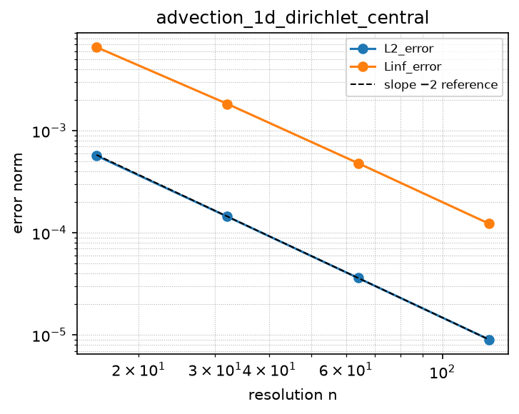
Convergence — case advection_1d_dirichlet_central
Error norms read from the committed golden tests/conformance/convergence/advection_1d_dirichlet_central/golden/errors.json (binding: julia; nothing recomputed for display).
| n | L2_error | observed order | Linf_error | observed order |
|---|---|---|---|---|
| 16 | 5.690e-04 | — | 6.559e-03 | — |
| 32 | 1.442e-04 | 1.98 | 1.829e-03 | 1.84 |
| 64 | 3.617e-05 | 2.00 | 4.809e-04 | 1.93 |
| 128 | 9.050e-06 | 2.00 | 1.232e-04 | 1.96 |
Expected order: 2 (± 0.2).
central_D1_periodic
Source: grids/cartesian_uniform_1d/rules/central_D1_periodic.esm
Rewrites ∂f/∂x — match pattern:
{"op": "D", "args": ["f"], "wrt": "x"}
where): fires only when f is a bare field shaped [x]. Under import-edge renaming (§9.7.7) the wrt literal and this shape follow the renamed axis together, so the rule can be imported more than once (each instance scoped to its own grid) without a first-declared-wins collision. A consumer differentiating a compound inline expression must bind it to a declared shaped observed first.Discretization — one makearray tiling the output axes; boundary conditions live in the face regions of this same rule (esm-spec §9.6.8; later regions overwrite earlier, §4.3.2):
| Region | Treatment | Value |
|---|---|---|
x ∈ [2, N−1] | interior | central_D1_interior(f)[i] = (f[i+1] − f[i−1]) / (2·dx) for i ∈ [2, N−1] |
x = 1 | boundary face | (f[2] − f[N]) / (2·dx) |
x = N | boundary face | (f[1] − f[N−1]) / (2·dx) |
Second-order centered first derivative with periodic boundary on cartesian_uniform_1d. Interior [2, N-1]: the imported 3-point centered stencil (f[i+1]-f[i-1])/(2 dx). Faces wrap periodically: the i=1 face uses the ghost f[0]=f[N], giving (f[2]-f[N])/(2 dx); the i=N face uses f[N+1]=f[1], giving (f[1]-f[N-1])/(2 dx). dx is a free name resolving to the consuming model’s spacing variable (the grid’s consumer-supplied geometry contract; see grids/cartesian_uniform_1d/grid.esm) — the periodic wrap is dx-scale-invariant, so the rule serves any domain extent unchanged. Matches plain D(f, wrt: x) at default priority, so compound rules (e.g. a second-derivative rule at priority 10) fire first, match-scoped with where: {f: {shape: [x]}} (esm-spec §9.6.1) so it fires only on the first derivative of a bare field over this grid’s x index set; under import-edge renaming (esm-spec §9.7.7) the wrt literal and the where shape follow the renamed axis together. O(dx^2). A model imports exactly one first-derivative rule for x (this centered rule or an upwind rule), never both.
References
- Fornberg, B. (1988). Generation of finite difference formulas on arbitrarily spaced grids. Mathematics of Computation 51(184), 699-706.
doi:10.1090/S0025-5718-1988-0935077-0
Conformance fixtures
- ast:
central_D1_periodic— statusactive - convergence:
advection_1d_periodic_central— statusactive - simulation:
advection_1d_periodic_central— statusactive
Convergence — case advection_1d_periodic_central
Error norms read from the committed golden tests/conformance/convergence/advection_1d_periodic_central/golden/errors.json (binding: julia; nothing recomputed for display).
| n | L2_error | observed order | Linf_error | observed order |
|---|---|---|---|---|
| 16 | 1.602e-02 | — | 1.602e-02 | — |
| 32 | 4.029e-03 | 1.99 | 4.022e-03 | 1.99 |
| 64 | 1.009e-03 | 2.00 | 1.009e-03 | 2.00 |
| 128 | 2.523e-04 | 2.00 | 2.523e-04 | 2.00 |
Expected order: 2 (± 0.2).
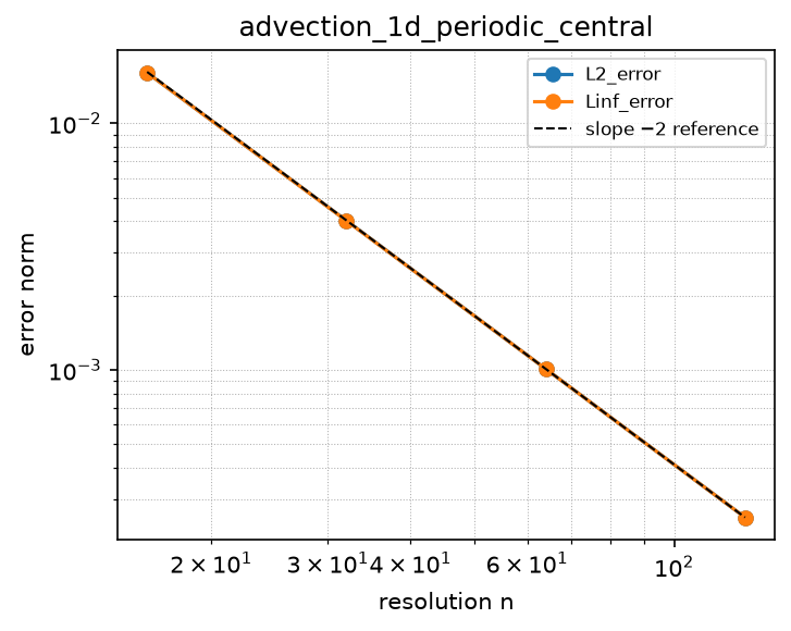
central_D1_zero_grad_bc
Source: grids/cartesian_uniform_1d/rules/central_D1_zero_grad_bc.esm
Rewrites ∂f/∂x — match pattern:
{"op": "D", "args": ["f"], "wrt": "x"}
where): fires only when f is a bare field shaped [x]. Under import-edge renaming (§9.7.7) the wrt literal and this shape follow the renamed axis together, so the rule can be imported more than once (each instance scoped to its own grid) without a first-declared-wins collision. A consumer differentiating a compound inline expression must bind it to a declared shaped observed first.Discretization — one makearray tiling the output axes; boundary conditions live in the face regions of this same rule (esm-spec §9.6.8; later regions overwrite earlier, §4.3.2):
| Region | Treatment | Value |
|---|---|---|
x ∈ [2, N−1] | interior | central_D1_interior(f)[i] = (f[i+1] − f[i−1]) / (2·dx) for i ∈ [2, N−1] |
x = 1 | boundary face | (4·f[2] − 3·f[1] − f[3]) / (2·dx) |
x = N | boundary face | ((f[N−2] − 4·f[N−1]) + 3·f[N]) / (2·dx) |
Second-order centered first derivative with zero-gradient (no-flux) boundary conditions on cartesian_uniform_1d. Interior [2, N-1]: the imported 3-point centered stencil (f[i+1]-f[i-1])/(2 dx). Faces i=1 and i=N use SECOND-ORDER one-sided (Fornberg) differences rather than a ghost reflection: i=1 = (-3 f[1] + 4 f[2] - f[3])/(2 dx) and i=N = (f[N-2] - 4 f[N-1] + 3 f[N])/(2 dx). The one-sided weights are the exact Fornberg (1988) coefficients for the first derivative at an edge node: _fornberg_weights(0, [0,1,2], 1) = [-3/2, 2, -1/2] (forward, i=1) and _fornberg_weights(0, [-2,-1,0], 1) = [1/2, -2, 3/2] (backward, i=N), each divided by dx. CHOICE OF FACE ORDER: unlike grids/latlon/rules/central_D_lat_zero_grad_bc, which closes its pole rows with a 1st-order one-sided difference (relying on the manufactured solution’s high pole-compatibility for superconvergence), this rule uses 2nd-order one-sided faces whose LOCAL truncation is O(dx^2), matching the interior stencil. That makes the operator robustly 2nd-order for ANY smooth field, without requiring the solution to have vanishing higher derivatives at the walls — the zero-gradient tag names the boundary CONTEXT (a no-flux wall) in which this centered gradient is used, not a ghost-reflection closure. dx is a free name resolving to the consuming model’s spacing variable (the grid’s consumer-supplied geometry contract; see grids/cartesian_uniform_1d/grid.esm) — the one-sided face stencils are dx-scale-invariant, so the rule serves any domain extent unchanged. Matches plain D(f, wrt: x) at default priority, so compound rules (e.g. a second-derivative rule at priority 10) fire first, match-scoped with where: {f: {shape: [x]}} (esm-spec 9.6.1) so it fires only on the first derivative of a bare field declared over this grid’s x index set (not on any unrelated D(., wrt: x) reusing the axis name); under import-edge renaming (esm-spec 9.7.7) the wrt literal and the where shape follow the renamed axis together, so two cartesian instances coexist scoped to their own grids. The constraint requires a bare shaped variable; a consumer differentiating a compound expression must bind it to a declared x-shaped observed first. O(dx^2). A model imports exactly one first-derivative rule for x (this centered zero-gradient rule, the periodic centered rule, or an upwind rule), never more than one.
References
- Fornberg, B. (1988). Generation of finite difference formulas on arbitrarily spaced grids. Mathematics of Computation 51(184), 699-706.
doi:10.1090/S0025-5718-1988-0935077-0
Conformance fixtures
- ast:
central_D1_zero_grad_bc— statusactive - convergence:
advection_1d_zero_grad_central— statusactive - simulation:
advection_1d_zero_grad_central— statusactive
Convergence — case advection_1d_zero_grad_central
Error norms read from the committed golden tests/conformance/convergence/advection_1d_zero_grad_central/golden/errors.json (binding: julia; nothing recomputed for display).
| n | L2_error | observed order | Linf_error | observed order |
|---|---|---|---|---|
| 16 | 3.581e-03 | — | 4.175e-03 | — |
| 32 | 8.247e-04 | 2.12 | 8.049e-04 | 2.38 |
| 64 | 2.032e-04 | 2.02 | 2.016e-04 | 2.00 |
| 128 | 5.065e-05 | 2.00 | 5.042e-05 | 2.00 |
Expected order: 2 (± 0.2).
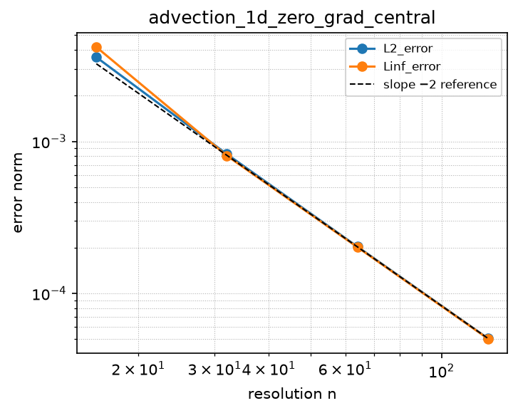
central_D2_4_dirichlet_bc
Source: grids/cartesian_uniform_1d/rules/central_D2_4_dirichlet_bc.esm
Rewrites ∂²f/∂x² at priority 10 — match pattern:
{"op": "D", "args": [{"op": "D", "args": ["f"], "wrt": "x"}], "wrt": "x"}
where): fires only when f is a bare field shaped [x]. Under import-edge renaming (§9.7.7) the wrt literal and this shape follow the renamed axis together, so the rule can be imported more than once (each instance scoped to its own grid) without a first-declared-wins collision. A consumer differentiating a compound inline expression must bind it to a declared shaped observed first.Discretization — one makearray tiling the output axes; boundary conditions live in the face regions of this same rule (esm-spec §9.6.8; later regions overwrite earlier, §4.3.2):
| Region | Treatment | Value |
|---|---|---|
x ∈ [3, N−2] | interior | central_D2_4_interior(f)[i] = (−f[i−2] + 16·f[i−1] − 30·f[i] + 16·f[i+1] − f[i+2]) / (12·dx·dx) for i ∈ [3, N−2] |
x = 1 | boundary face | central_D2_4_dirichlet_face1(gL, f[1], f[2], f[3], f[4], f[5]) = (2560·g + −4095·f1 + 1848·f2 + −378·f3 + 72·f4 + −7·f5)/(756·dx·dx) |
x = 2 | boundary face | central_D2_4_dirichlet_face2(gL, f[1], f[2], f[3], f[4], f[5]) = (−256·g + 1323·f1 + −2100·f2 + 1134·f3 + −108·f4 + 7·f5)/(756·dx·dx) |
x = N−1 | boundary face | central_D2_4_dirichlet_face2(gR, f[N], f[N−1], f[N−2], f[N−3], f[N−4]) = (−256·g + 1323·f1 + −2100·f2 + 1134·f3 + −108·f4 + 7·f5)/(756·dx·dx) |
x = N | boundary face | central_D2_4_dirichlet_face1(gR, f[N], f[N−1], f[N−2], f[N−3], f[N−4]) = (2560·g + −4095·f1 + 1848·f2 + −378·f3 + 72·f4 + −7·f5)/(756·dx·dx) |
Fourth-order centered second derivative with inhomogeneous Dirichlet (fixed-value) boundaries on cartesian_uniform_1d, cell-centered. Interior [3, N-2]: the imported 5-point fourth-order stencil central_D2_4_interior, (-f[i-2] + 16 f[i-1] - 30 f[i] + 16 f[i+1] - f[i+2])/(12 dx^2), O(dx^4). The four near-boundary rows i in {1, 2, N-1, N}, whose centered 5-point stencils would reach outside the domain, are closed with the imported one-sided fourth-order face templates central_D2_4_dirichlet_face1 (nearest-wall row) and central_D2_4_dirichlet_face2 (second row): each is the unique degree-5 polynomial through the prescribed wall value and the five nearest cell values, differentiated twice at that cell. The wall values gL (left wall x=x0) and gR (right wall x=x0+N*dx) are consumer-supplied free names bound into the face templates (the g parameter); the same free-name contract as the grid geometry dx (grids/cartesian_uniform_1d/grid.esm). A consuming model declares gL/gR as ordinary real parameters; a parameter not overridden falls back to its default (esm-spec 6: default, or 0), so gL=gR=0 is the homogeneous-Dirichlet case. gL/gR appear only in the runtime rule body, never in build-time ic/reference positions (AGENTS.md build-time scope caveat). The right wall reuses the same face weights by reflection (the second derivative is even under x -> -x), so f1..f5 there map to cells N, N-1, N-2, N-3, N-4 (increasing distance from the right wall) and g binds to gR. Because BOTH the interior stencil and all four boundary closures are O(dx^4), the global scheme is uniformly fourth order with no boundary reduction; a steady linear profile carrying the wall values is discretely exact at every row (all closure weight-sums are zero). Verified stable for the heat operator: the homogeneous discrete Laplacian’s spectrum lies in the left half plane (largest real part -pi^2, the fundamental Dirichlet mode). Compound match on D(D(f,x),x) at priority 10 (esm-spec 9.6.3 compound precedence), match-scoped with where: {f: {shape: [x]}} (esm-spec 9.6.1) so it fires only on the second derivative of a bare field declared over this grid’s x index set; under import-edge renaming (esm-spec 9.7.7) the wrt literals and the where shape follow the renamed axis together. A model imports exactly one second-derivative rule for x.
References
- Fornberg, B. (1988). Generation of finite difference formulas on arbitrarily spaced grids. Mathematics of Computation 51(184), 699-706.
doi:10.1090/S0025-5718-1988-0935077-0 - LeVeque, R. J. (2007). Finite Difference Methods for Ordinary and Partial Differential Equations. SIAM. Section 2.12 (boundary conditions; one-sided high-order closures).
Conformance fixtures
- ast:
central_D2_4_dirichlet_bc— statusactive - convergence:
heat_1d_dirichlet_o4— statusactive - simulation:
heat_1d_dirichlet_o4— statusactive
Convergence — case heat_1d_dirichlet_o4
Error norms read from the committed golden tests/conformance/convergence/heat_1d_dirichlet_o4/golden/errors.json (binding: julia; nothing recomputed for display).
| n | L2_error | observed order | Linf_error | observed order |
|---|---|---|---|---|
| 8 | 9.756e-07 | — | 2.500e-06 | — |
| 16 | 6.667e-08 | 3.87 | 1.601e-07 | 3.96 |
| 32 | 4.225e-09 | 3.98 | 1.007e-08 | 3.99 |
| 64 | 2.647e-10 | 4.00 | 6.301e-10 | 4.00 |
Expected order: 4 (± 0.2).
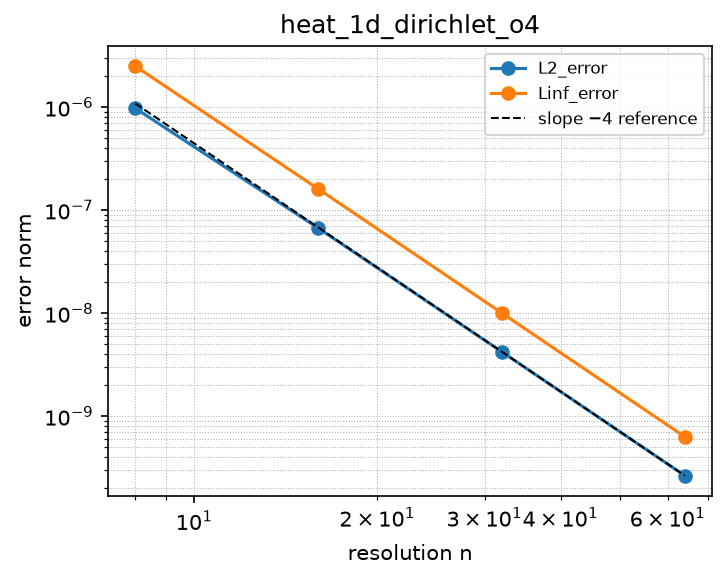
central_D2_4_neumann_bc
Source: grids/cartesian_uniform_1d/rules/central_D2_4_neumann_bc.esm
Rewrites ∂²f/∂x² at priority 10 — match pattern:
{"op": "D", "args": [{"op": "D", "args": ["f"], "wrt": "x"}], "wrt": "x"}
where): fires only when f is a bare field shaped [x]. Under import-edge renaming (§9.7.7) the wrt literal and this shape follow the renamed axis together, so the rule can be imported more than once (each instance scoped to its own grid) without a first-declared-wins collision. A consumer differentiating a compound inline expression must bind it to a declared shaped observed first.Discretization — one makearray tiling the output axes; boundary conditions live in the face regions of this same rule (esm-spec §9.6.8; later regions overwrite earlier, §4.3.2):
| Region | Treatment | Value |
|---|---|---|
x ∈ [3, N−2] | interior | central_D2_4_interior(f)[i] = (−f[i−2] + 16·f[i−1] − 30·f[i] + 16·f[i+1] − f[i+2]) / (12·dx·dx) for i ∈ [3, N−2] |
x = 1 | boundary face | central_D2_4_neumann_face1(qL, f[1], f[2], f[3], f[4], f[5]) = (−1.92×10⁴·q·dx + −1.5285×10⁴·f1 + 7544·f2 + 1.2546×10⁴·f3 + −5784·f4 + 979·f5)/(2.0268×10⁴·dx·dx) |
x = 2 | boundary face | central_D2_4_neumann_face2(qL, f[1], f[2], f[3], f[4], f[5]) = (1920·q·dx + 2.6019×10⁴·f1 + −5.21×10⁴·f2 + 2.8134×10⁴·f3 + −2124·f4 + 71·f5)/(2.0268×10⁴·dx·dx) |
x = N−1 | boundary face | central_D2_4_neumann_face2(−qR, f[N], f[N−1], f[N−2], f[N−3], f[N−4]) = (1920·q·dx + 2.6019×10⁴·f1 + −5.21×10⁴·f2 + 2.8134×10⁴·f3 + −2124·f4 + 71·f5)/(2.0268×10⁴·dx·dx) |
x = N | boundary face | central_D2_4_neumann_face1(−qR, f[N], f[N−1], f[N−2], f[N−3], f[N−4]) = (−1.92×10⁴·q·dx + −1.5285×10⁴·f1 + 7544·f2 + 1.2546×10⁴·f3 + −5784·f4 + 979·f5)/(2.0268×10⁴·dx·dx) |
Fourth-order centered second derivative with inhomogeneous Neumann (fixed-flux) boundaries on cartesian_uniform_1d, cell-centered. Interior [3, N-2]: the imported 5-point fourth-order stencil central_D2_4_interior, (-f[i-2] + 16 f[i-1] - 30 f[i] + 16 f[i+1] - f[i+2])/(12 dx^2), O(dx^4). The four near-boundary rows i in {1, 2, N-1, N}, whose centered 5-point stencils would reach outside the domain, are closed with the imported one-sided fourth-order face templates central_D2_4_neumann_face1 (nearest-wall row) and central_D2_4_neumann_face2 (second row): each is the unique degree-5 Hermite-type polynomial matching the prescribed wall derivative and the five nearest cell values, differentiated twice at that cell. The wall gradients qL (df/dx at the left wall x=x0, +x direction) and qR (df/dx at the right wall x=x0+N*dx, +x direction) are consumer-supplied free names; the same free-name contract as the grid geometry dx (grids/cartesian_uniform_1d/grid.esm). A consuming model declares qL/qR as ordinary real parameters; a parameter not overridden falls back to its default (esm-spec 6: default, or 0), so qL=qR=0 is the homogeneous (zero-flux) case and the rule reduces exactly to a zero-gradient fourth-order closure. qL/qR appear only in the runtime rule body, never in build-time ic/reference positions (AGENTS.md build-time scope caveat). The left face templates take the wall derivative datum q as their +x-into-domain slope, so the left rows bind q -> qL. The right wall reuses the SAME face weights by reflection (the second derivative is even under x -> -x while df/dx is odd), so the right rows bind q -> -qR and map f1..f5 to cells N, N-1, N-2, N-3, N-4 (increasing distance from the right wall). Because BOTH the interior stencil and all four boundary closures are O(dx^4), the global scheme is uniformly fourth order with no boundary reduction; a steady ramp carrying the wall fluxes is discretely exact at every row (the value-weight sums are zero and the derivative term supplies the exact wall slope). Verified stable for the heat operator: the homogeneous discrete Laplacian’s spectrum lies in the closed left half plane with a single zero eigenvalue (the constant Neumann nullspace), exactly as the continuous pure-Neumann Laplacian. Compound match on D(D(f,x),x) at priority 10 (esm-spec 9.6.3 compound precedence), match-scoped with where: {f: {shape: [x]}} (esm-spec 9.6.1) so it fires only on the second derivative of a bare field declared over this grid’s x index set; under import-edge renaming (esm-spec 9.7.7) the wrt literals and the where shape follow the renamed axis together. A model imports exactly one second-derivative rule for x.
References
- Fornberg, B. (1988). Generation of finite difference formulas on arbitrarily spaced grids. Mathematics of Computation 51(184), 699-706.
doi:10.1090/S0025-5718-1988-0935077-0 - LeVeque, R. J. (2007). Finite Difference Methods for Ordinary and Partial Differential Equations. SIAM. Section 2.12 (Neumann boundary conditions; one-sided high-order closures).
Conformance fixtures
- ast:
central_D2_4_neumann_bc— statusactive - convergence:
heat_1d_neumann_flux_o4— statusactive - simulation:
heat_1d_neumann_flux_o4— statusactive
Convergence — case heat_1d_neumann_flux_o4
Error norms read from the committed golden tests/conformance/convergence/heat_1d_neumann_flux_o4/golden/errors.json (binding: julia; nothing recomputed for display).
| n | L2_error | observed order | Linf_error | observed order |
|---|---|---|---|---|
| 8 | 5.784e-06 | — | 7.277e-06 | — |
| 16 | 3.045e-07 | 4.25 | 5.105e-07 | 3.83 |
| 32 | 1.334e-08 | 4.51 | 2.546e-08 | 4.33 |
| 64 | 6.376e-10 | 4.39 | 8.525e-10 | 4.90 |
Expected order: 4 (± 0.5).
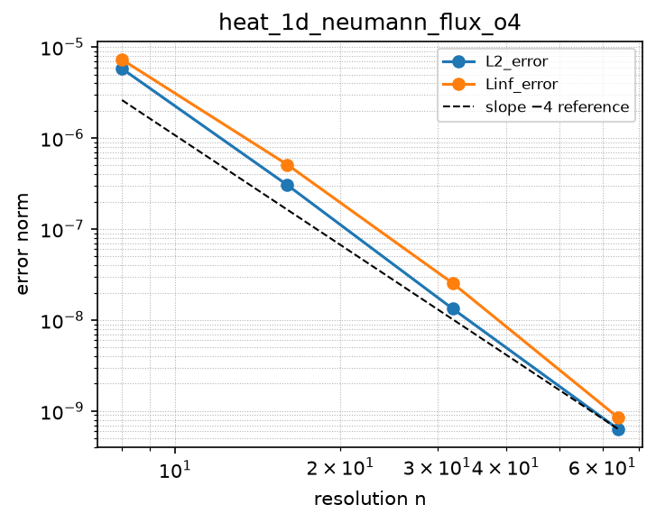
central_D2_4_periodic
Source: grids/cartesian_uniform_1d/rules/central_D2_4_periodic.esm
Rewrites ∂²f/∂x² at priority 10 — match pattern:
{"op": "D", "args": [{"op": "D", "args": ["f"], "wrt": "x"}], "wrt": "x"}
where): fires only when f is a bare field shaped [x]. Under import-edge renaming (§9.7.7) the wrt literal and this shape follow the renamed axis together, so the rule can be imported more than once (each instance scoped to its own grid) without a first-declared-wins collision. A consumer differentiating a compound inline expression must bind it to a declared shaped observed first.Discretization — one makearray tiling the output axes; boundary conditions live in the face regions of this same rule (esm-spec §9.6.8; later regions overwrite earlier, §4.3.2):
| Region | Treatment | Value |
|---|---|---|
x ∈ [3, N−2] | interior | central_D2_4_interior(f)[i] = (−f[i−2] + 16·f[i−1] − 30·f[i] + 16·f[i+1] − f[i+2]) / (12·dx·dx) for i ∈ [3, N−2] |
x = 1 | boundary face | (−f[N−1] + 16·f[N] − 30·f[1] + 16·f[2] − f[3]) / (12·dx·dx) |
x = 2 | boundary face | (−f[N] + 16·f[1] − 30·f[2] + 16·f[3] − f[4]) / (12·dx·dx) |
x = N−1 | boundary face | (−f[N−3] + 16·f[N−2] − 30·f[N−1] + 16·f[N] − f[1]) / (12·dx·dx) |
x = N | boundary face | (−f[N−2] + 16·f[N−1] − 30·f[N] + 16·f[1] − f[2]) / (12·dx·dx) |
Fourth-order centered second derivative with periodic boundary on cartesian_uniform_1d. Compound match on D(D(f,x),x) at priority 10, so it fires on the whole second derivative before any plain-D rule lowers the inner derivative (esm-spec 9.6.3 compound precedence), match-scoped with where: {f: {shape: [x]}} (esm-spec 9.6.1); under import-edge renaming (esm-spec 9.7.7) the wrt literals and the where shape follow the renamed axis together. Interior [3, N-2]: the imported 5-point stencil (-f[i-2] + 16 f[i-1] - 30 f[i] + 16 f[i+1] - f[i+2]) / (12 dx^2). The four near-boundary rows i in {1, 2, N-1, N} carry the same 5-point weights with the out-of-range neighbors wrapped periodically (i-2, i-1 wrap past 1 to N-1, N; i+1, i+2 wrap past N to 1, 2), so the whole operator is the exact circulant 4th-order Laplacian — O(dx^4) with no boundary order reduction, the natural high-order analogue of central_D1_periodic. dx is a free name resolving to the consuming model’s spacing variable (grids/cartesian_uniform_1d/grid.esm); the periodic wrap is dx-scale-invariant. A model imports exactly one second-derivative rule for x.
References
- Fornberg, B. (1988). Generation of finite difference formulas on arbitrarily spaced grids. Mathematics of Computation 51(184), 699-706.
doi:10.1090/S0025-5718-1988-0935077-0
Conformance fixtures
- ast:
central_D2_4_periodic— statusactive - convergence:
heat_1d_periodic_o4— statusactive - simulation:
heat_1d_periodic_o4— statusactive
Convergence — case heat_1d_periodic_o4
Error norms read from the committed golden tests/conformance/convergence/heat_1d_periodic_o4/golden/errors.json (binding: julia; nothing recomputed for display).
| n | L2_error | observed order | Linf_error | observed order |
|---|---|---|---|---|
| 8 | 1.580e-04 | — | 1.403e-04 | — |
| 16 | 1.029e-05 | 3.94 | 9.701e-06 | 3.85 |
| 32 | 6.497e-07 | 3.99 | 6.216e-07 | 3.96 |
| 64 | 4.071e-08 | 4.00 | 3.909e-08 | 3.99 |
Expected order: 4 (± 0.2).
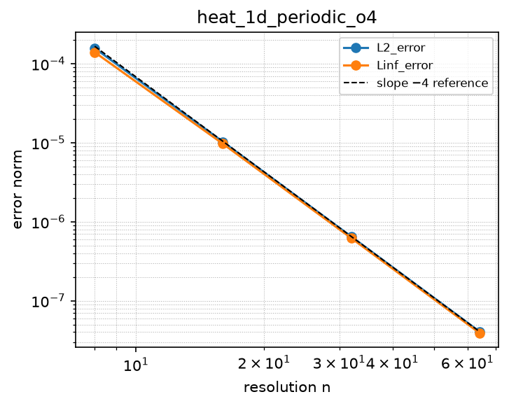
central_D2_6_dirichlet_bc
Source: grids/cartesian_uniform_1d/rules/central_D2_6_dirichlet_bc.esm
Rewrites ∂²f/∂x² at priority 10 — match pattern:
{"op": "D", "args": [{"op": "D", "args": ["f"], "wrt": "x"}], "wrt": "x"}
where): fires only when f is a bare field shaped [x]. Under import-edge renaming (§9.7.7) the wrt literal and this shape follow the renamed axis together, so the rule can be imported more than once (each instance scoped to its own grid) without a first-declared-wins collision. A consumer differentiating a compound inline expression must bind it to a declared shaped observed first.Discretization — one makearray tiling the output axes; boundary conditions live in the face regions of this same rule (esm-spec §9.6.8; later regions overwrite earlier, §4.3.2):
| Region | Treatment | Value |
|---|---|---|
x ∈ [4, N−3] | interior | central_D2_6_interior(f)[i] = (2·f[i−3] − 27·f[i−2] + 270·f[i−1] − 490·f[i] + 270·f[i+1] − 27·f[i+2] + 2·f[i+3]) / (180·dx·dx) for i ∈ [4, N−3] |
x = 1 | boundary face | central_D2_6_dirichlet_face1(gL, f[1], f[2], f[3], f[4], f[5], f[6], f[7]) = (8.6016×10⁴·g + −1.36136×10⁵·f1 + 5.6628×10⁴·f2 + −3861·f3 + −5720·f4 + 4290·f5 + −1404·f6 + 187·f7)/(2.574×10⁴·dx·dx) |
x = 2 | boundary face | central_D2_6_dirichlet_face2(gL, f[1], f[2], f[3], f[4], f[5], f[6], f[7]) = (−2048·g + 1.1349×10⁴·f1 + −1.7745×10⁴·f2 + 8073·f3 + 1170·f4 + −1105·f5 + 351·f6 + −45·f7)/(7020·dx·dx) |
x = 3 | boundary face | central_D2_6_dirichlet_face3(gL, f[1], f[2], f[3], f[4], f[5], f[6], f[7]) = (4096·g + −1.7589×10⁴·f1 + 1.21836×10⁵·f2 + −2.16216×10⁵·f3 + 1.2012×10⁵·f4 + −1.3585×10⁴·f5 + 1404·f6 + −66·f7)/(7.722×10⁴·dx·dx) |
x = N−2 | boundary face | central_D2_6_dirichlet_face3(gR, f[N], f[N−1], f[N−2], f[N−3], f[N−4], f[N−5], f[N−6]) = (4096·g + −1.7589×10⁴·f1 + 1.21836×10⁵·f2 + −2.16216×10⁵·f3 + 1.2012×10⁵·f4 + −1.3585×10⁴·f5 + 1404·f6 + −66·f7)/(7.722×10⁴·dx·dx) |
x = N−1 | boundary face | central_D2_6_dirichlet_face2(gR, f[N], f[N−1], f[N−2], f[N−3], f[N−4], f[N−5], f[N−6]) = (−2048·g + 1.1349×10⁴·f1 + −1.7745×10⁴·f2 + 8073·f3 + 1170·f4 + −1105·f5 + 351·f6 + −45·f7)/(7020·dx·dx) |
x = N | boundary face | central_D2_6_dirichlet_face1(gR, f[N], f[N−1], f[N−2], f[N−3], f[N−4], f[N−5], f[N−6]) = (8.6016×10⁴·g + −1.36136×10⁵·f1 + 5.6628×10⁴·f2 + −3861·f3 + −5720·f4 + 4290·f5 + −1404·f6 + 187·f7)/(2.574×10⁴·dx·dx) |
Sixth-order centered second derivative with inhomogeneous Dirichlet (fixed-value) boundaries on cartesian_uniform_1d, cell-centered. Interior [4, N-3]: the imported 7-point sixth-order stencil central_D2_6_interior, (2 f[i-3] - 27 f[i-2] + 270 f[i-1] - 490 f[i] + 270 f[i+1] - 27 f[i+2] + 2 f[i+3])/(180 dx^2), O(dx^6). The six near-boundary rows i in {1, 2, 3, N-2, N-1, N}, whose centered 7-point stencils would reach outside the domain, are closed with the imported one-sided sixth-order face templates central_D2_6_dirichlet_face1 (nearest-wall row), face2 (second row) and face3 (third row): each is the unique degree-7 polynomial through the prescribed wall value and the seven nearest cell values, differentiated twice at that cell. The wall values gL (left wall x=x0) and gR (right wall x=x0+N*dx) are consumer-supplied free names bound into the face templates (the g parameter); the same free-name contract as the grid geometry dx (grids/cartesian_uniform_1d/grid.esm). A consuming model declares gL/gR as ordinary real parameters; a parameter not overridden falls back to its default (esm-spec 6: default, or 0), so gL=gR=0 is the homogeneous-Dirichlet case. gL/gR appear only in the runtime rule body, never in build-time ic/reference positions (AGENTS.md build-time scope caveat). The right wall reuses the same face weights by reflection (the second derivative is even under x -> -x), so f1..f7 there map to cells N, N-1, N-2, N-3, N-4, N-5, N-6 (increasing distance from the right wall) and g binds to gR. Requires N >= 7 so the interior 7-point stencil and the seven-cell boundary closures have distinct points; the six boundary rows plus the interior [4,N-3] tile [1,N] exactly. Because BOTH the interior stencil and all six boundary closures are derived to be O(dx^6) (each exact for polynomials up to degree 7; every closure weight-sum is zero so a steady linear profile carrying the wall values is discretely exact at every row), the design order is uniformly six; the honestly observed order of accuracy on the heat MMS sweep is pinned in tests/conformance/convergence/heat_1d_dirichlet_o6. Verified stable for the heat operator: the homogeneous discrete Laplacian’s spectrum is real and negative with largest real part exactly -pi^2 (the fundamental Dirichlet mode), so it lies strictly in the left half plane. Compound match on D(D(f,x),x) at priority 10 (esm-spec 9.6.3 compound precedence), match-scoped with where: {f: {shape: [x]}} (esm-spec 9.6.1) so it fires only on the second derivative of a bare field declared over this grid’s x index set; under import-edge renaming (esm-spec 9.7.7) the wrt literals and the where shape follow the renamed axis together. A model imports exactly one second-derivative rule for x.
References
- Fornberg, B. (1988). Generation of finite difference formulas on arbitrarily spaced grids. Mathematics of Computation 51(184), 699-706.
doi:10.1090/S0025-5718-1988-0935077-0 - LeVeque, R. J. (2007). Finite Difference Methods for Ordinary and Partial Differential Equations. SIAM. Section 2.12 (boundary conditions; one-sided high-order closures).
Conformance fixtures
- ast:
central_D2_6_dirichlet_bc— statusactive - convergence:
heat_1d_dirichlet_o6— statusactive
Convergence — case heat_1d_dirichlet_o6
Error norms read from the committed golden tests/conformance/convergence/heat_1d_dirichlet_o6/golden/errors.json (binding: julia; nothing recomputed for display).
| n | L2_error | observed order | Linf_error | observed order |
|---|---|---|---|---|
| 8 | 7.259e-08 | — | 1.873e-07 | — |
| 16 | 4.874e-10 | 7.22 | 9.892e-10 | 7.56 |
| 32 | 6.520e-12 | 6.22 | 1.558e-11 | 5.99 |
| 64 | 1.422e-13 | 5.52 | 1.044e-12 | 3.90 |
Expected order: 6 (± 0.6).
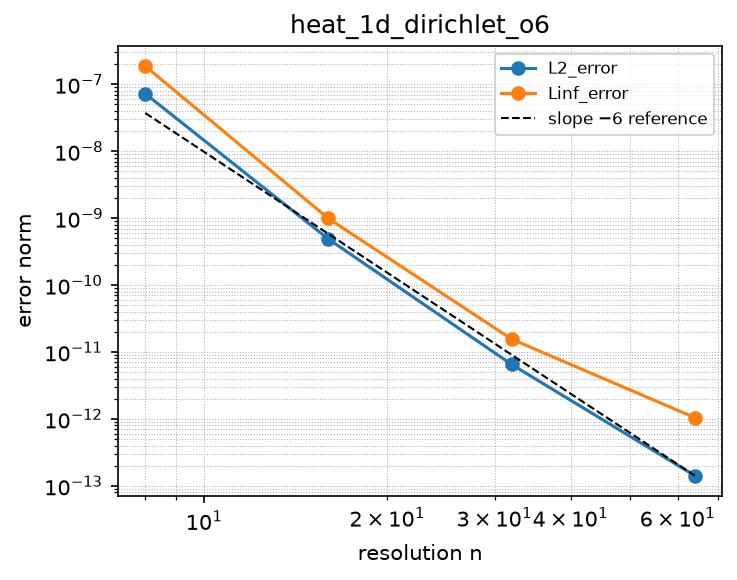
central_D2_6_neumann_bc
Source: grids/cartesian_uniform_1d/rules/central_D2_6_neumann_bc.esm
Rewrites ∂²f/∂x² at priority 10 — match pattern:
{"op": "D", "args": [{"op": "D", "args": ["f"], "wrt": "x"}], "wrt": "x"}
where): fires only when f is a bare field shaped [x]. Under import-edge renaming (§9.7.7) the wrt literal and this shape follow the renamed axis together, so the rule can be imported more than once (each instance scoped to its own grid) without a first-declared-wins collision. A consumer differentiating a compound inline expression must bind it to a declared shaped observed first.Discretization — one makearray tiling the output axes; boundary conditions live in the face regions of this same rule (esm-spec §9.6.8; later regions overwrite earlier, §4.3.2):
| Region | Treatment | Value |
|---|---|---|
x ∈ [4, N−3] | interior | central_D2_6_interior(f)[i] = (2·f[i−3] − 27·f[i−2] + 270·f[i−1] − 490·f[i] + 270·f[i+1] − 27·f[i+2] + 2·f[i+3]) / (180·dx·dx) for i ∈ [4, N−3] |
x = 1 | boundary face | central_D2_6_neumann_face1(qL, f[1], f[2], f[3], f[4], f[5], f[6], f[7]) = (−1.354752×10⁷·q·dx + −4.382308×10⁶·f1 + −1.80976×10⁷·f2 + 4.529776×10⁷·f3 + −3.595516×10⁷·f4 + 1.735677×10⁷·f5 + −4.804812×10⁶·f6 + 5.85341×10⁵·f7)/(1.585242×10⁷·dx·dx) |
x = 2 | boundary face | central_D2_6_neumann_face2(qL, f[1], f[2], f[3], f[4], f[5], f[6], f[7]) = (1.18272×10⁶·q·dx + 1.869115×10⁷·f1 + −3.544678×10⁷·f2 + 1.406812×10⁷·f3 + 5.47347×10⁶·f4 + −3.779905×10⁶·f5 + 1.136601×10⁶·f6 + −1.42665×10⁵·f7)/(1.585242×10⁷·dx·dx) |
x = 3 | boundary face | central_D2_6_neumann_face3(qL, f[1], f[2], f[3], f[4], f[5], f[6], f[7]) = (−2.1504×10⁵·q·dx + −2.349569×10⁶·f1 + 2.417076×10⁷·f2 + −4.363002×10⁷·f3 + 2.414452×10⁷·f4 + −2.555285×10⁶·f5 + 2.25684×10⁵·f6 + −6086·f7)/(1.585242×10⁷·dx·dx) |
x = N−2 | boundary face | central_D2_6_neumann_face3(−qR, f[N], f[N−1], f[N−2], f[N−3], f[N−4], f[N−5], f[N−6]) = (−2.1504×10⁵·q·dx + −2.349569×10⁶·f1 + 2.417076×10⁷·f2 + −4.363002×10⁷·f3 + 2.414452×10⁷·f4 + −2.555285×10⁶·f5 + 2.25684×10⁵·f6 + −6086·f7)/(1.585242×10⁷·dx·dx) |
x = N−1 | boundary face | central_D2_6_neumann_face2(−qR, f[N], f[N−1], f[N−2], f[N−3], f[N−4], f[N−5], f[N−6]) = (1.18272×10⁶·q·dx + 1.869115×10⁷·f1 + −3.544678×10⁷·f2 + 1.406812×10⁷·f3 + 5.47347×10⁶·f4 + −3.779905×10⁶·f5 + 1.136601×10⁶·f6 + −1.42665×10⁵·f7)/(1.585242×10⁷·dx·dx) |
x = N | boundary face | central_D2_6_neumann_face1(−qR, f[N], f[N−1], f[N−2], f[N−3], f[N−4], f[N−5], f[N−6]) = (−1.354752×10⁷·q·dx + −4.382308×10⁶·f1 + −1.80976×10⁷·f2 + 4.529776×10⁷·f3 + −3.595516×10⁷·f4 + 1.735677×10⁷·f5 + −4.804812×10⁶·f6 + 5.85341×10⁵·f7)/(1.585242×10⁷·dx·dx) |
Sixth-order centered second derivative with inhomogeneous Neumann (fixed-flux) boundaries on cartesian_uniform_1d, cell-centered. Interior [4, N-3]: the imported 7-point sixth-order stencil central_D2_6_interior, (2 f[i-3] - 27 f[i-2] + 270 f[i-1] - 490 f[i] + 270 f[i+1] - 27 f[i+2] + 2 f[i+3])/(180 dx^2), O(dx^6). The six near-boundary rows i in {1, 2, 3, N-2, N-1, N}, whose centered 7-point stencils would reach outside the domain, are closed with the imported one-sided sixth-order face templates central_D2_6_neumann_face1 (nearest-wall row), face2 (second row) and face3 (third row): each is the unique degree-7 Hermite-type polynomial matching the prescribed wall derivative and the seven nearest cell values, differentiated twice at that cell. The wall gradients qL (df/dx at the left wall x=x0, +x direction) and qR (df/dx at the right wall x=x0+N*dx, +x direction) are consumer-supplied free names; the same free-name contract as the grid geometry dx (grids/cartesian_uniform_1d/grid.esm). A consuming model declares qL/qR as ordinary real parameters; a parameter not overridden falls back to its default (esm-spec 6: default, or 0), so qL=qR=0 is the homogeneous (zero-flux) case and the rule reduces exactly to a zero-gradient sixth-order closure. qL/qR appear only in the runtime rule body, never in build-time ic/reference positions (AGENTS.md build-time scope caveat). The left face templates take the wall derivative datum q as their +x-into-domain slope, so the left rows bind q -> qL. The right wall reuses the SAME face weights by reflection (the second derivative is even under x -> -x while df/dx is odd), so the right rows bind q -> -qR and map f1..f7 to cells N, N-1, N-2, N-3, N-4, N-5, N-6 (increasing distance from the right wall). Requires N >= 7 so the interior 7-point stencil and the seven-cell boundary closures have distinct points; the six boundary rows plus the interior [4,N-3] tile [1,N] exactly. Because BOTH the interior stencil and all six boundary closures are derived to be O(dx^6) (each exact for polynomials up to degree 7; every value-weight sum is zero and the derivative term supplies the exact wall slope, so a steady ramp carrying the wall fluxes is discretely exact at every row), the design order is uniformly six; the honestly observed order of accuracy on the heat MMS sweep is pinned in tests/conformance/convergence/heat_1d_neumann_flux_o6. Verified stable for the heat operator: the homogeneous discrete Laplacian’s spectrum lies in the closed left half plane with a single zero eigenvalue (the constant Neumann nullspace) and second-largest real part exactly -pi^2, exactly as the continuous pure-Neumann Laplacian. Compound match on D(D(f,x),x) at priority 10 (esm-spec 9.6.3 compound precedence), match-scoped with where: {f: {shape: [x]}} (esm-spec 9.6.1) so it fires only on the second derivative of a bare field declared over this grid’s x index set; under import-edge renaming (esm-spec 9.7.7) the wrt literals and the where shape follow the renamed axis together. A model imports exactly one second-derivative rule for x.
References
- Fornberg, B. (1988). Generation of finite difference formulas on arbitrarily spaced grids. Mathematics of Computation 51(184), 699-706.
doi:10.1090/S0025-5718-1988-0935077-0 - LeVeque, R. J. (2007). Finite Difference Methods for Ordinary and Partial Differential Equations. SIAM. Section 2.12 (Neumann boundary conditions; one-sided high-order closures).
Conformance fixtures
- ast:
central_D2_6_neumann_bc— statusactive - convergence:
heat_1d_neumann_flux_o6— statusactive
Convergence — case heat_1d_neumann_flux_o6
Error norms read from the committed golden tests/conformance/convergence/heat_1d_neumann_flux_o6/golden/errors.json (binding: julia; nothing recomputed for display).
| n | L2_error | observed order | Linf_error | observed order |
|---|---|---|---|---|
| 8 | 4.103e-07 | — | 5.246e-07 | — |
| 16 | 7.840e-09 | 5.71 | 1.434e-08 | 5.19 |
| 32 | 8.493e-11 | 6.53 | 2.120e-10 | 6.08 |
| 64 | 7.665e-13 | 6.79 | 2.183e-12 | 6.60 |
Expected order: 6 (± 0.6).
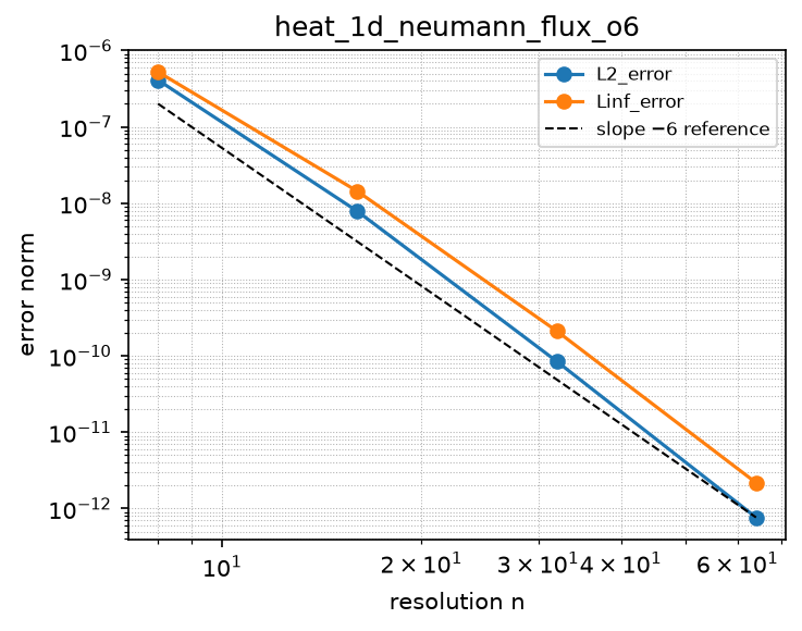
central_D2_6_periodic
Source: grids/cartesian_uniform_1d/rules/central_D2_6_periodic.esm
Rewrites ∂²f/∂x² at priority 10 — match pattern:
{"op": "D", "args": [{"op": "D", "args": ["f"], "wrt": "x"}], "wrt": "x"}
where): fires only when f is a bare field shaped [x]. Under import-edge renaming (§9.7.7) the wrt literal and this shape follow the renamed axis together, so the rule can be imported more than once (each instance scoped to its own grid) without a first-declared-wins collision. A consumer differentiating a compound inline expression must bind it to a declared shaped observed first.Discretization — one makearray tiling the output axes; boundary conditions live in the face regions of this same rule (esm-spec §9.6.8; later regions overwrite earlier, §4.3.2):
| Region | Treatment | Value |
|---|---|---|
x ∈ [4, N−3] | interior | central_D2_6_interior(f)[i] = (2·f[i−3] − 27·f[i−2] + 270·f[i−1] − 490·f[i] + 270·f[i+1] − 27·f[i+2] + 2·f[i+3]) / (180·dx·dx) for i ∈ [4, N−3] |
x = 1 | boundary face | (2·f[N−2] − 27·f[N−1] + 270·f[N] − 490·f[1] + 270·f[2] − 27·f[3] + 2·f[4]) / (180·dx·dx) |
x = 2 | boundary face | (2·f[N−1] − 27·f[N] + 270·f[1] − 490·f[2] + 270·f[3] − 27·f[4] + 2·f[5]) / (180·dx·dx) |
x = 3 | boundary face | (2·f[N] − 27·f[1] + 270·f[2] − 490·f[3] + 270·f[4] − 27·f[5] + 2·f[6]) / (180·dx·dx) |
x = N−2 | boundary face | (2·f[N−5] − 27·f[N−4] + 270·f[N−3] − 490·f[N−2] + 270·f[N−1] − 27·f[N] + 2·f[1]) / (180·dx·dx) |
x = N−1 | boundary face | (2·f[N−4] − 27·f[N−3] + 270·f[N−2] − 490·f[N−1] + 270·f[N] − 27·f[1] + 2·f[2]) / (180·dx·dx) |
x = N | boundary face | (2·f[N−3] − 27·f[N−2] + 270·f[N−1] − 490·f[N] + 270·f[1] − 27·f[2] + 2·f[3]) / (180·dx·dx) |
Sixth-order centered second derivative with periodic boundary on cartesian_uniform_1d. Compound match on D(D(f,x),x) at priority 10, so it fires on the whole second derivative before any plain-D rule lowers the inner derivative (esm-spec 9.6.3 compound precedence), match-scoped with where: {f: {shape: [x]}} (esm-spec 9.6.1); under import-edge renaming (esm-spec 9.7.7) the wrt literals and the where shape follow the renamed axis together. Interior [4, N-3]: the imported 7-point stencil (2 f[i-3] - 27 f[i-2] + 270 f[i-1] - 490 f[i] + 270 f[i+1] - 27 f[i+2] + 2 f[i+3]) / (180 dx^2). The six near-boundary rows i in {1, 2, 3, N-2, N-1, N} carry the same 7-point weights with out-of-range neighbors wrapped periodically, so the whole operator is the exact circulant 6th-order Laplacian — O(dx^6) with no boundary order reduction. Requires N >= 7 for the 7-point stencil to have distinct points. dx is a free name resolving to the consuming model’s spacing variable (grids/cartesian_uniform_1d/grid.esm); the periodic wrap is dx-scale-invariant. A model imports exactly one second-derivative rule for x.
References
- Fornberg, B. (1988). Generation of finite difference formulas on arbitrarily spaced grids. Mathematics of Computation 51(184), 699-706.
doi:10.1090/S0025-5718-1988-0935077-0
Conformance fixtures
- ast:
central_D2_6_periodic— statusactive - convergence:
heat_1d_periodic_o6— statusactive
Convergence — case heat_1d_periodic_o6
Error norms read from the committed golden tests/conformance/convergence/heat_1d_periodic_o6/golden/errors.json (binding: julia; nothing recomputed for display).
| n | L2_error | observed order | Linf_error | observed order |
|---|---|---|---|---|
| 8 | 1.503e-05 | — | 1.335e-05 | — |
| 16 | 2.524e-07 | 5.90 | 2.380e-07 | 5.81 |
| 32 | 4.016e-09 | 5.97 | 3.842e-09 | 5.95 |
Expected order: 6 (± 0.3).
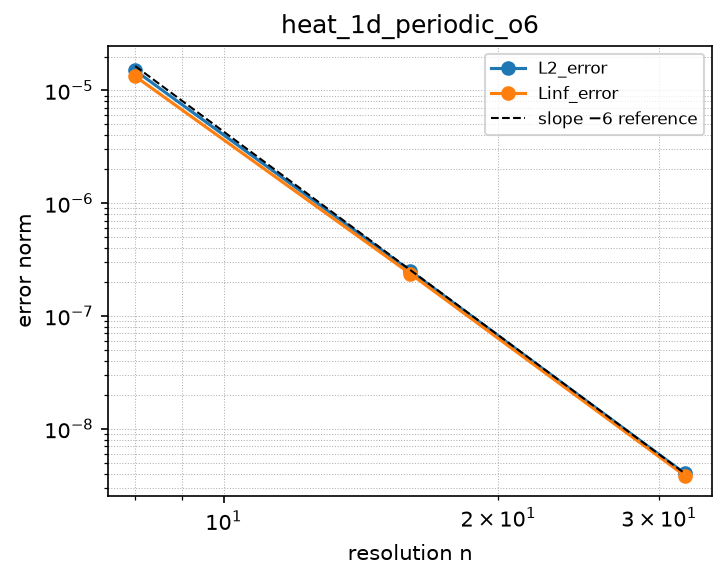
central_D2_dirichlet_bc
Source: grids/cartesian_uniform_1d/rules/central_D2_dirichlet_bc.esm
Rewrites ∂²f/∂x² at priority 10 — match pattern:
{"op": "D", "args": [{"op": "D", "args": ["f"], "wrt": "x"}], "wrt": "x"}
where): fires only when f is a bare field shaped [x]. Under import-edge renaming (§9.7.7) the wrt literal and this shape follow the renamed axis together, so the rule can be imported more than once (each instance scoped to its own grid) without a first-declared-wins collision. A consumer differentiating a compound inline expression must bind it to a declared shaped observed first.Discretization — one makearray tiling the output axes; boundary conditions live in the face regions of this same rule (esm-spec §9.6.8; later regions overwrite earlier, §4.3.2):
| Region | Treatment | Value |
|---|---|---|
x ∈ [2, N−1] | interior | central_D2_interior(f)[i] = (f[i+1] − 2·f[i] + f[i−1]) / dx² for i ∈ [2, N−1] |
x = 1 | boundary face | ((f[2] − 3·f[1]) + 2·gL) / dx² |
x = N | boundary face | ((f[N−1] − 3·f[N]) + 2·gR) / dx² |
Second-order centered second derivative with inhomogeneous Dirichlet (fixed-value) boundary conditions on cartesian_uniform_1d, cell-centered. Interior [2, N-1]: the imported 3-point stencil. Faces i=1 and i=N: mirror-ghost elimination against a prescribed wall value. gL and gR are consumer-supplied free names (the same free-name contract as the grid geometry dx; see grids/cartesian_uniform_1d/grid.esm) giving the field value at the left wall x=x0 and the right wall x=x0+Ndx. On this cell-centered grid the wall sits half a cell outside the first center, so linear reconstruction to the wall gives the ghost f[0]=2gL-f[1] (and f[N+1]=2gR-f[N]); substituting into the 3-point stencil yields D2[1] = (f[2]-3f[1]+2gL)/dx^2 and D2[N] = (f[N-1]-3f[N]+2*gR)/dx^2. A consuming model declares gL/gR as ordinary real parameters; a parameter not overridden falls back to its default (esm-spec §6: default, or 0), so gL=gR=0 is the homogeneous-Dirichlet case. The gL/gR terms live only in the runtime rule body, never in build-time ic/reference positions (AGENTS.md build-time scope caveat). Compound match on D(D(f,x),x) at priority 10 (esm-spec §9.6.3), match-scoped with where: {f: {shape: [x]}} (esm-spec §9.6.1) so it fires only on the second derivative of a bare field over this grid’s x index set; under import-edge renaming (esm-spec §9.7.7) the wrt literals and the where shape follow the renamed axis together. Interior O(dx^2); the one-sided mirror-ghost faces preserve global 2nd-order convergence for Dirichlet-compatible solutions.
References
- LeVeque, R. J. (2007). Finite Difference Methods for Ordinary and Partial Differential Equations. SIAM. Section 2.12 (boundary conditions; cell-centered Dirichlet via mirror ghost).
Conformance fixtures
- ast:
central_D2_dirichlet_bc— statusactive - convergence:
advection_1d_dirichlet_central— statusactive - convergence:
heat_1d_dirichlet— statusactive - simulation:
advection_1d_dirichlet_central— statusactive - simulation:
heat_1d_dirichlet— statusactive
Convergence — case advection_1d_dirichlet_central
Error norms read from the committed golden tests/conformance/convergence/advection_1d_dirichlet_central/golden/errors.json (binding: julia; nothing recomputed for display).
| n | L2_error | observed order | Linf_error | observed order |
|---|---|---|---|---|
| 16 | 5.690e-04 | — | 6.559e-03 | — |
| 32 | 1.442e-04 | 1.98 | 1.829e-03 | 1.84 |
| 64 | 3.617e-05 | 2.00 | 4.809e-04 | 1.93 |
| 128 | 9.050e-06 | 2.00 | 1.232e-04 | 1.96 |
Expected order: 2 (± 0.2).
Convergence — case heat_1d_dirichlet
Error norms read from the committed golden tests/conformance/convergence/heat_1d_dirichlet/golden/errors.json (binding: julia; nothing recomputed for display).
| n | L2_error | observed order | Linf_error | observed order |
|---|---|---|---|---|
| 16 | 1.317e-05 | — | 3.121e-05 | — |
| 32 | 3.296e-06 | 2.00 | 7.837e-06 | 1.99 |
| 64 | 8.241e-07 | 2.00 | 1.962e-06 | 2.00 |
| 128 | 2.060e-07 | 2.00 | 4.906e-07 | 2.00 |
Expected order: 2 (± 0.2).
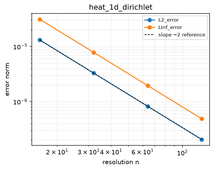
central_D2_neumann_bc
Source: grids/cartesian_uniform_1d/rules/central_D2_neumann_bc.esm
Rewrites ∂²f/∂x² at priority 10 — match pattern:
{"op": "D", "args": [{"op": "D", "args": ["f"], "wrt": "x"}], "wrt": "x"}
where): fires only when f is a bare field shaped [x]. Under import-edge renaming (§9.7.7) the wrt literal and this shape follow the renamed axis together, so the rule can be imported more than once (each instance scoped to its own grid) without a first-declared-wins collision. A consumer differentiating a compound inline expression must bind it to a declared shaped observed first.Discretization — one makearray tiling the output axes; boundary conditions live in the face regions of this same rule (esm-spec §9.6.8; later regions overwrite earlier, §4.3.2):
| Region | Treatment | Value |
|---|---|---|
x ∈ [2, N−1] | interior | central_D2_interior(f)[i] = (f[i+1] − 2·f[i] + f[i−1]) / dx² for i ∈ [2, N−1] |
x = 1 | boundary face | (f[2] − f[1] − qL·dx) / dx² |
x = N | boundary face | ((f[N−1] − f[N]) + qR·dx) / dx² |
Second-order centered second derivative with inhomogeneous Neumann (fixed-flux) boundary conditions on cartesian_uniform_1d. Interior [2, N-1]: the imported 3-point stencil. Faces i=1 and i=N: ghost elimination against a prescribed wall gradient. qL and qR are consumer-supplied free names (the same keyed-factor / free-name contract as the grid geometry dx; see grids/cartesian_uniform_1d/grid.esm) giving the value of df/dx (in the +x direction) at the left wall x=x0 and the right wall x=x0+Ndx respectively. A consuming model declares them as ordinary real parameters; a parameter not overridden falls back to its default (esm-spec §6: default, or 0), so the homogeneous case is the zero default and this rule reduces exactly to central_D2_zero_grad_bc when qL=qR=0. Ghost elimination: (f[1]-f[0])/dx = qL gives f[0]=f[1]-qLdx, so D2[1] = (f[2]-f[1]-qLdx)/dx^2; (f[N+1]-f[N])/dx = qR gives f[N+1]=f[N]+qRdx, so D2[N] = (f[N-1]-f[N]+qR*dx)/dx^2. The qL/qR terms live only in the runtime rule body, never in build-time ic/reference positions, so the consumer-scope free-name resolution is well-defined (AGENTS.md build-time scope caveat). Compound match on D(D(f,x),x) at priority 10 (esm-spec §9.6.3 compound precedence), match-scoped with where: {f: {shape: [x]}} (esm-spec §9.6.1) so it fires only on the second derivative of a bare field declared over this grid’s x index set; under import-edge renaming (esm-spec §9.7.7) the wrt literals and the where shape follow the renamed axis together. Interior O(dx^2); the one-sided faces are O(dx) locally, preserving global 2nd-order convergence for Neumann-compatible solutions.
References
- LeVeque, R. J. (2007). Finite Difference Methods for Ordinary and Partial Differential Equations. SIAM. Section 2.12 (Neumann boundary conditions by ghost-point elimination).
Conformance fixtures
- ast:
central_D2_neumann_bc— statusactive - convergence:
heat_1d_neumann_flux— statusactive - simulation:
heat_1d_neumann_flux— statusactive
Convergence — case heat_1d_neumann_flux
Error norms read from the committed golden tests/conformance/convergence/heat_1d_neumann_flux/golden/errors.json (binding: julia; nothing recomputed for display).
| n | L2_error | observed order | Linf_error | observed order |
|---|---|---|---|---|
| 16 | 3.411e-05 | — | 3.121e-05 | — |
| 32 | 8.538e-06 | 2.00 | 7.837e-06 | 1.99 |
| 64 | 2.135e-06 | 2.00 | 1.962e-06 | 2.00 |
| 128 | 5.338e-07 | 2.00 | 4.905e-07 | 2.00 |
Expected order: 2 (± 0.2).
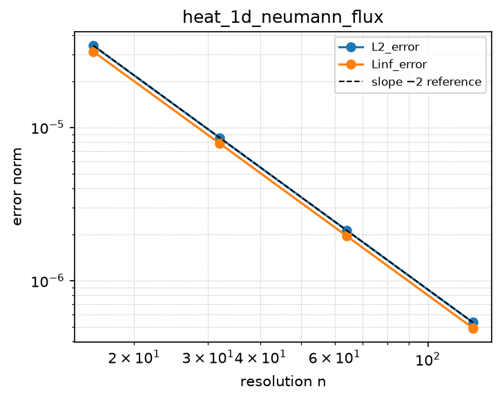
central_D2_periodic
Source: grids/cartesian_uniform_1d/rules/central_D2_periodic.esm
Rewrites ∂²f/∂x² at priority 10 — match pattern:
{"op": "D", "args": [{"op": "D", "args": ["f"], "wrt": "x"}], "wrt": "x"}
where): fires only when f is a bare field shaped [x]. Under import-edge renaming (§9.7.7) the wrt literal and this shape follow the renamed axis together, so the rule can be imported more than once (each instance scoped to its own grid) without a first-declared-wins collision. A consumer differentiating a compound inline expression must bind it to a declared shaped observed first.Discretization — one makearray tiling the output axes; boundary conditions live in the face regions of this same rule (esm-spec §9.6.8; later regions overwrite earlier, §4.3.2):
| Region | Treatment | Value |
|---|---|---|
x ∈ [2, N−1] | interior | central_D2_interior(f)[i] = (f[i+1] − 2·f[i] + f[i−1]) / dx² for i ∈ [2, N−1] |
x = 1 | boundary face | (f[2] − 2·f[1] + f[N]) / dx² |
x = N | boundary face | (f[1] − 2·f[N] + f[N−1]) / dx² |
Second-order centered second derivative with periodic boundary on cartesian_uniform_1d. Compound match on D(D(f,x),x) at priority 10, so it fires on the whole second derivative before any plain-D rule lowers the inner derivative (esm-spec 9.6.3 compound precedence), match-scoped with where: {f: {shape: [x]}} (esm-spec 9.6.1) so it fires only on the second derivative of a bare field declared over this grid’s x index set (not on any unrelated D(D(.,x),x) reusing the axis name); under import-edge renaming (esm-spec 9.7.7) the wrt literals and the where shape follow the renamed axis together, so two cartesian instances coexist scoped to their own grids. The constraint requires a bare shaped variable; a consumer differentiating a compound inner expression must bind it to a declared x-shaped observed first. Interior [2, N-1]: the imported 3-point stencil (f[i+1] - 2 f[i] + f[i-1]) / dx^2. The two faces i=1 and i=N carry the same 3-point weights [1, -2, 1] with the out-of-range neighbor wrapped periodically (i=1 uses the ghost f[0]=f[N], giving (f[2] - 2 f[1] + f[N]) / dx^2; i=N uses f[N+1]=f[1], giving (f[1] - 2 f[N] + f[N-1]) / dx^2), so the whole operator is the exact circulant 3-point Laplacian — O(dx^2) with no boundary order reduction, the natural second-order analogue of central_D1_periodic and the low-order companion of central_D2_4_periodic / central_D2_6_periodic. dx is a free name resolving to the consuming model’s spacing variable (grids/cartesian_uniform_1d/grid.esm); the periodic wrap is dx-scale-invariant, so the rule serves any domain extent unchanged. A model imports exactly one second-derivative rule for x.
References
- Fornberg, B. (1988). Generation of finite difference formulas on arbitrarily spaced grids. Mathematics of Computation 51(184), 699-706.
doi:10.1090/S0025-5718-1988-0935077-0
Conformance fixtures
- ast:
central_D2_periodic— statusactive - convergence:
heat_1d_periodic— statusactive - simulation:
heat_1d_periodic— statusactive
Convergence — case heat_1d_periodic
Error norms read from the committed golden tests/conformance/convergence/heat_1d_periodic/golden/errors.json (binding: julia; nothing recomputed for display).
| n | L2_error | observed order | Linf_error | observed order |
|---|---|---|---|---|
| 8 | 1.990e-03 | — | 1.767e-03 | — |
| 16 | 5.049e-04 | 1.98 | 4.760e-04 | 1.89 |
| 32 | 1.267e-04 | 1.99 | 1.212e-04 | 1.97 |
| 64 | 3.170e-05 | 2.00 | 3.044e-05 | 1.99 |
Expected order: 2 (± 0.2).
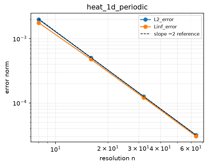
central_D2_zero_grad_bc
Source: grids/cartesian_uniform_1d/rules/central_D2_zero_grad_bc.esm
Rewrites ∂²f/∂x² at priority 10 — match pattern:
{"op": "D", "args": [{"op": "D", "args": ["f"], "wrt": "x"}], "wrt": "x"}
where): fires only when f is a bare field shaped [x]. Under import-edge renaming (§9.7.7) the wrt literal and this shape follow the renamed axis together, so the rule can be imported more than once (each instance scoped to its own grid) without a first-declared-wins collision. A consumer differentiating a compound inline expression must bind it to a declared shaped observed first.Discretization — one makearray tiling the output axes; boundary conditions live in the face regions of this same rule (esm-spec §9.6.8; later regions overwrite earlier, §4.3.2):
| Region | Treatment | Value |
|---|---|---|
x ∈ [2, N−1] | interior | central_D2_interior(f)[i] = (f[i+1] − 2·f[i] + f[i−1]) / dx² for i ∈ [2, N−1] |
x = 1 | boundary face | (f[2] − f[1]) / dx² |
x = N | boundary face | (f[N−1] − f[N]) / dx² |
Second-order centered second derivative with zero-gradient (homogeneous Neumann) boundary conditions on cartesian_uniform_1d. Compound match on D(D(f,x),x) at priority 10, so it fires on the whole second derivative before any plain-D rule lowers the inner derivative (esm-spec 9.6.3 compound precedence), match-scoped with where: {f: {shape: [x]}} (esm-spec 9.6.1) so it fires only on the second derivative of a bare field declared over this grid’s x index set (not on any unrelated D(D(.,x),x) reusing the axis name); under import-edge renaming (esm-spec 9.7.7) the wrt literals and the where shape follow the renamed axis together, so two cartesian instances coexist scoped to their own grids. The constraint requires a bare shaped variable; a consumer differentiating a compound inner expression must bind it to a declared x-shaped observed first. Interior [2, N-1]: the imported 3-point stencil. Faces i=1 and i=N: ghost elimination with f[0]=f[1] and f[N+1]=f[N], giving (f[2]-f[1])/dx^2 and (f[N-1]-f[N])/dx^2. dx is a free name resolving to the consuming model’s spacing variable (the grid’s consumer-supplied geometry contract; see grids/cartesian_uniform_1d/grid.esm) — the zero-gradient ghost elimination itself is dx-scale-invariant, so the rule serves any domain extent unchanged. Interior O(dx^2); the one-sided faces are O(dx) locally, which preserves global 2nd-order convergence for zero-gradient-compatible solutions.
References
- LeVeque, R. J. (2007). Finite Difference Methods for Ordinary and Partial Differential Equations. SIAM. Section 2.12 (Neumann boundary conditions by ghost-point elimination).
Conformance fixtures
- ast:
central_D2_zero_grad_bc— statusactive - ast:
e2e_consuming_model— statusactive - ast:
two_cartesian_grids_coexist— statusactive - convergence:
heat_1d_zero_grad— statusactive - convergence:
heat_1d_zero_grad_nonunit— statusactive - simulation:
heat_1d_zero_grad— statusactive - simulation:
heat_1d_zero_grad_nonunit— statusactive - simulation:
two_cartesian_grids_coexist— statusactive
Convergence — case heat_1d_zero_grad
Error norms read from the committed golden tests/conformance/convergence/heat_1d_zero_grad/golden/errors.json (binding: julia; nothing recomputed for display).
| n | L2_error | observed order | Linf_error | observed order |
|---|---|---|---|---|
| 16 | 3.167e-05 | — | 3.121e-05 | — |
| 32 | 7.925e-06 | 2.00 | 7.837e-06 | 1.99 |
| 64 | 1.982e-06 | 2.00 | 1.962e-06 | 2.00 |
| 128 | 4.954e-07 | 2.00 | 4.905e-07 | 2.00 |
Expected order: 2 (± 0.2).
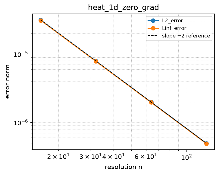
Convergence — case heat_1d_zero_grad_nonunit
Error norms read from the committed golden tests/conformance/convergence/heat_1d_zero_grad_nonunit/golden/errors.json (binding: julia; nothing recomputed for display).
| n | L2_error | observed order | Linf_error | observed order |
|---|---|---|---|---|
| 16 | 3.959e-05 | — | 3.891e-05 | — |
| 32 | 9.906e-06 | 2.00 | 9.773e-06 | 1.99 |
| 64 | 2.477e-06 | 2.00 | 2.446e-06 | 2.00 |
| 128 | 6.193e-07 | 2.00 | 6.117e-07 | 2.00 |
Expected order: 2 (± 0.2).
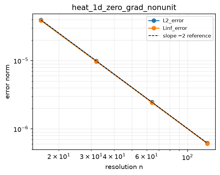
flux_limiter_minmod_D_inflow_bc
Source: grids/cartesian_uniform_1d/rules/flux_limiter_minmod_D_inflow_bc.esm
Rewrites ∂u/∂x at priority 10 — match pattern:
{"op": "D", "args": ["u"], "wrt": "x"}
where): fires only when u is a bare field shaped [x]. Under import-edge renaming (§9.7.7) the wrt literal and this shape follow the renamed axis together, so the rule can be imported more than once (each instance scoped to its own grid) without a first-declared-wins collision. A consumer differentiating a compound inline expression must bind it to a declared shaped observed first.Discretization — one makearray tiling the output axes; boundary conditions live in the face regions of this same rule (esm-spec §9.6.8; later regions overwrite earlier, §4.3.2):
| Region | Treatment | Value |
|---|---|---|
x ∈ [3, N−1] | interior | flux_limiter_minmod_D_interior(u)[i] = (flux_limiter_minmod_flux(f[i−1], f[i], f[i+1]) − flux_limiter_minmod_flux(f[i−2], f[i−1], f[i])) / dx for i ∈ [3, N−1] |
x = 1 | boundary face | (flux_limiter_minmod_flux(gL, u[1], u[2]) − gL) / dx |
x = 2 | boundary face | (flux_limiter_minmod_flux(u[1], u[2], u[3]) − flux_limiter_minmod_flux(gL, u[1], u[2])) / dx |
x = N | boundary face | (flux_limiter_minmod_flux(u[N−1], u[N], u[N]) − flux_limiter_minmod_flux(u[N−2], u[N−1], u[N])) / dx |
Second-order TVD minmod flux-limited finite-VOLUME advective first derivative u_x with OPEN boundaries – a prescribed inflow (Dirichlet) value at the upstream (left) wall and a one-sided extrapolation (outflow) closure at the downstream (right) wall – on cartesian_uniform_1d, for scalar linear advection with non-negative transport speed (a consumer writes u_t = -cD(u, wrt: x), c >= 0). This is the open-boundary sibling of rules/flux_limiter_minmod_D_periodic.esm and, unlike that ~55 KB inlined periodic file, is built THINLY on extracted stencils: the interior is a single apply of stencils/flux_limiter_minmod_D_interior.esm (which composes stencils/flux_limiter_minmod_flux.esm over stencils/minmod2.esm, the reusable minmod kernel), and the boundary faces reuse the SAME flux stencil with ghost bindings – the good compositional pattern (mirroring rules/ppm_D_periodic over stencils/ppm_D_interior + ppm_flux, and rules/lax_friedrichs_D_inflow_bc over its interior + flux). The semi-discrete divergence is D u[i] = (G_{i+1/2} - G_{i-1/2})/dx with the minmod-limited face flux G(um1,u0,up1) = u0 + 0.5minmod(u0 - um1, up1 - u0) (u0 the upwind cell, +x). Self-contained makearray over axis x with FOUR regions: interior [3, N-1] is the imported flux-difference aggregate; the three faces i=1, i=2, i=N reach a ghost. INFLOW (left, i=1 and the i=2 left face): the wall face flux is G_{1/2} = gL (first-order upwind: the prescribed inflow value carried into the domain, the only defensible value where the reconstruction would need the absent cell u[-1]), and the u[0] ghost that the limited face G_{3/2} = flux(gL, u[1], u[2]) needs is injected as the inflow value gL; so D u[1] = (flux(gL,u[1],u[2]) - gL)/dx and D u[2] = (flux(u[1],u[2],u[3]) - flux(gL,u[1],u[2]))/dx. Near the smooth inflow the limiter stays active (gL is a genuine one-sided slope), degrading to first-order upwind only at the wall face itself where the stencil runs out – standard TVD boundary practice. OUTFLOW (right, i=N): the right ghost is set by ZEROTH-ORDER EXTRAPOLATION u[N+1] = u[N], so G_{N+1/2} = flux(u[N-1], u[N], u[N]); its upper slope Dp = u[N+1] - u[N] = 0 makes minmod(Dm, 0) EXACTLY 0, so the outflow face collapses to first-order upwind G_{N+1/2} = u[N] – carrying no external data and injecting no spurious reflection (non-reflecting). The one-sided upwind/limiter closure keeps pure advection well-posed with a single upstream wall value; a two-sided fixed-value closure would over-determine the outflow. gL is a free name with default 0 (the same consumer-supplied contract as rules/upwind1_D_inflow_bc’s gL and rules/lax_friedrichs_D_inflow_bc’s gL, and the grid geometry dx; grids/cartesian_uniform_1d/grid.esm): a consuming model declares gL as an ordinary real parameter giving the field value carried into the domain at the left wall x = x0, and an unset parameter falls back to its default (esm-spec 6; 0 = zero inflow). The gL term lives only in the runtime rule body, never in build-time ic/reference positions (AGENTS.md build-time scope caveat). dx is likewise the grid’s consumer-supplied free name; every face is dx-scale-invariant so the rule serves any domain extent unchanged. Second-order TVD where the limiter is inactive (the interior of a smooth monotone profile), monotonicity-preserving (no new extrema); the boundary faces are a formally first-order closure, but for a compatible smooth solution (exact inflow value, zero wall gradient) their residual is higher order, so the observed order approaches the design second order (norm-dependent, median ~1.9 L2 / ~1.8 Linf on the reference MMS) and is pinned honestly in tests/conformance/convergence/advection_1d_inflow_minmod. MATCH: plain D(u, wrt: x) at priority 10 (mirroring the periodic limiter sibling), match-scoped where: {u: {shape: [x]}} (esm-spec 9.6.1) so it fires only on the first derivative of a bare field over this grid’s x index set; under import-edge renaming (esm-spec 9.7.7) the wrt literal and the where shape follow the renamed axis together, so two cartesian instances coexist. The constraint requires a bare shaped variable. A model imports exactly one advection rule for x. Sign convention: upwind for flow in +x (inflow at the left wall).
References
- Roe, P. L. (1986). Characteristic-based schemes for the Euler equations. Ann. Rev. Fluid Mech. 18:337-365 (minmod eq. 35).
doi:10.1146/annurev.fl.18.010186.002005 - Sweby, P. K. (1984). High resolution schemes using flux limiters for hyperbolic conservation laws. SIAM J. Numer. Anal. 21(5):995-1011.
doi:10.1137/0721062 - LeVeque, R. J. (2002). Finite Volume Methods for Hyperbolic Problems. Cambridge University Press. Section 6.11-6.12 (flux-limiter methods) and eq. (6.35); Section 7 (inflow / outflow boundary conditions for advection).
Conformance fixtures
- ast:
flux_limiter_minmod_D_inflow_bc— statusactive - convergence:
advection_1d_inflow_minmod— statusactive - simulation:
advection_1d_inflow_minmod— statusactive
Convergence — case advection_1d_inflow_minmod
Error norms read from the committed golden tests/conformance/convergence/advection_1d_inflow_minmod/golden/errors.json (binding: julia; nothing recomputed for display).
| n | L2_error | observed order | Linf_error | observed order |
|---|---|---|---|---|
| 16 | 5.195e-03 | — | 8.626e-03 | — |
| 32 | 1.494e-03 | 1.80 | 2.931e-03 | 1.56 |
| 64 | 4.050e-04 | 1.88 | 8.653e-04 | 1.76 |
| 128 | 1.054e-04 | 1.94 | 2.240e-04 | 1.95 |
Expected order: 1.8 (± 0.2).
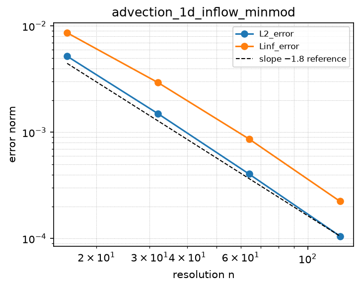
flux_limiter_minmod_D_periodic
Source: grids/cartesian_uniform_1d/rules/flux_limiter_minmod_D_periodic.esm
Rewrites ∂u/∂x at priority 10 — match pattern:
{"op": "D", "args": ["u"], "wrt": "x"}
where): fires only when u is a bare field shaped [x]. Under import-edge renaming (§9.7.7) the wrt literal and this shape follow the renamed axis together, so the rule can be imported more than once (each instance scoped to its own grid) without a first-declared-wins collision. A consumer differentiating a compound inline expression must bind it to a declared shaped observed first.Discretization — one makearray tiling the output axes; boundary conditions live in the face regions of this same rule (esm-spec §9.6.8; later regions overwrite earlier, §4.3.2):
| Region | Treatment | Value |
|---|---|---|
x ∈ [3, N−1] | interior | (u[i] + 0.5·(max(0, min(u[i] − u[i−1], u[i+1] − u[i])) + min(0, max(u[i] − u[i−1], u[i+1] − u[i]))) − (u[i−1] + 0.5·(max(0, min(u[i−1] − u[i−2], u[i] − u[i−1])) + min(0, max(u[i−1] − u[i−2], u[i] − u[i−1]))))) / dx for i ∈ [3, N−1] |
x = 1 | boundary face | (u[1] + 0.5·(max(0, min(u[1] − u[N], u[2] − u[1])) + min(0, max(u[1] − u[N], u[2] − u[1]))) − (u[N] + 0.5·(max(0, min(u[N] − u[N−1], u[1] − u[N])) + min(0, max(u[N] − u[N−1], u[1] − u[N]))))) / dx |
x = 2 | boundary face | (u[2] + 0.5·(max(0, min(u[2] − u[1], u[3] − u[2])) + min(0, max(u[2] − u[1], u[3] − u[2]))) − (u[1] + 0.5·(max(0, min(u[1] − u[N], u[2] − u[1])) + min(0, max(u[1] − u[N], u[2] − u[1]))))) / dx |
x = N | boundary face | (u[N] + 0.5·(max(0, min(u[N] − u[N−1], u[1] − u[N])) + min(0, max(u[N] − u[N−1], u[1] − u[N]))) − (u[N−1] + 0.5·(max(0, min(u[N−1] − u[N−2], u[N] − u[N−1])) + min(0, max(u[N−1] − u[N−2], u[N] − u[N−1]))))) / dx |
Second-order TVD flux-limited (minmod limiter) finite-VOLUME discretization of the advective first derivative u_x for scalar linear advection u_t = -c u_x (non-negative speed c, periodic) on cartesian_uniform_1d, in semi-discrete method-of-lines form. The consumer writes u_t = -cD(u, wrt: x); this rule emits the c-independent flux-difference D_i = (G[i+1/2] - G[i-1/2]) / dx that, scaled by -c, gives the finite-volume tendency with the high-resolution TVD flux F[i+1/2] = cu_i + 0.5cphi(r_i)(u_{i+1} - u_i), where phi(r) = max(0, min(1, r)) is the minmod limiter of Roe (1986) and r_i = (u_i - u_{i-1})/(u_{i+1} - u_i) is the upwind-to-local slope ratio (LeVeque 2002, eq. 6.35, in the dt->0 semi-discrete limit where the (1 - nu) Courant factor -> 1). Because c > 0 the flux factors as F = cG with G[i+1/2] = u_i + 0.5phi(r_i)(u_{i+1} - u_i), the c-free form emitted here (the +x sign is baked as in upwind1_D_periodic). DIVISION-FREE GUARD: the ratio r_i divides by (u_{i+1} - u_i), which vanishes at extrema and flat regions. Rather than form r explicitly (a 0/0 at flat data), the anti-diffusive correction 0.5phi(r_i)(u_{i+1} - u_i) is written in the algebraically-identical division-free jump form 0.5minmod(u_i - u_{i-1}, u_{i+1} - u_i), with the two-slope minmod expressed in pure max/min as minmod(a, b) = max(0, min(a, b)) + min(0, max(a, b)) (verified to machine precision against phi(r)(u_{i+1}-u_i) wherever r is defined, and finite — an exact 0 — when the jump is 0). This is the min/max form that avoids the explicit division a naive r would introduce; no epsilon regularization is needed. TVD, monotonicity-preserving (develops no new extrema; total variation non-increasing). Formally second-order accurate where the limiter is inactive (smooth monotone regions); the minmod limiter CLIPS at smooth extrema, so on a periodic sin the observed order of accuracy is below 2 (documented honestly in the convergence case — L2 ~1.6, Linf ~1.2). MATCH: plain D(u, wrt: x) at priority 10, match-scoped where: {u: {shape: [x]}} (esm-spec 9.6.1); the priority + shape constraint disambiguate it from a sibling plain first-derivative rule if both are ever in scope, and survive import-edge renaming (esm-spec 9.7.7). A model imports exactly one advection rule for x. Self-contained makearray: the TVD stencil is 4-point (u[i-2], u[i-1], u[i], u[i+1]) because the two face fluxes each need the upwind slope one cell back; interior [3, N-1] holds the flux-difference aggregate, and the three faces i=1, i=2, i=N carry the same flux difference with the out-of-range neighbors wrapped PERIODICALLY (i=1: u[0]=u[N], u[-1]=u[N-1]; i=2: u[0]=u[N]; i=N: u[N+1]=u[1]). dx is a free name resolving to the consuming model’s spacing variable (grids/cartesian_uniform_1d/grid.esm consumer-supplied geometry contract); the periodic wrap is dx-scale-invariant.
References
- Roe, P. L. (1986). Characteristic-based schemes for the Euler equations. Ann. Rev. Fluid Mech. 18:337-365 (minmod eq. 35, superbee eq. 36).
doi:10.1146/annurev.fl.18.010186.002005 - Sweby, P. K. (1984). High resolution schemes using flux limiters for hyperbolic conservation laws. SIAM J. Numer. Anal. 21(5):995-1011.
doi:10.1137/0721062 - LeVeque, R. J. (2002). Finite Volume Methods for Hyperbolic Problems. Cambridge University Press. Section 6.11-6.12 (flux-limiter methods) and eq. (6.35); Chapter 4 (Lax-Friedrichs / Rusanov).
Conformance fixtures
- ast:
flux_limiter_minmod_D_periodic— statusactive - convergence:
advection_1d_periodic_minmod— statusactive - simulation:
advection_1d_periodic_minmod— statusactive
Convergence — case advection_1d_periodic_minmod
Error norms read from the committed golden tests/conformance/convergence/advection_1d_periodic_minmod/golden/errors.json (binding: julia; nothing recomputed for display).
| n | L2_error | observed order | Linf_error | observed order |
|---|---|---|---|---|
| 16 | 4.370e-02 | — | 6.007e-02 | — |
| 32 | 1.479e-02 | 1.56 | 2.720e-02 | 1.14 |
| 64 | 4.815e-03 | 1.62 | 1.153e-02 | 1.24 |
| 128 | 1.554e-03 | 1.63 | 4.599e-03 | 1.33 |
Expected order: 1.43 (± 0.25).
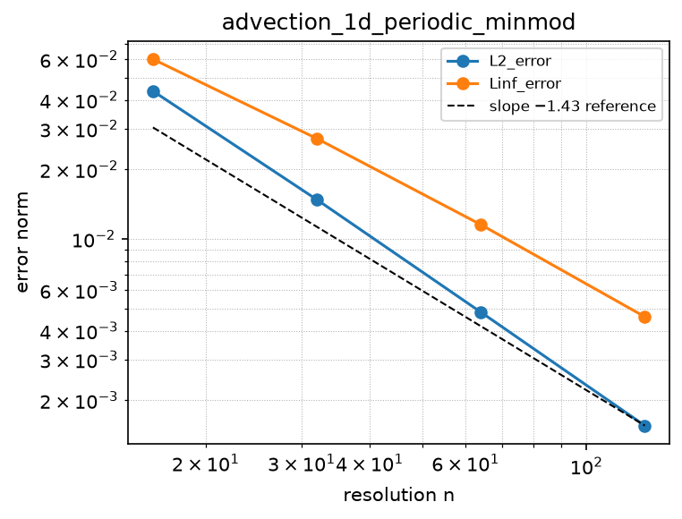
flux_limiter_superbee_D_inflow_bc
Source: grids/cartesian_uniform_1d/rules/flux_limiter_superbee_D_inflow_bc.esm
Rewrites ∂u/∂x at priority 10 — match pattern:
{"op": "D", "args": ["u"], "wrt": "x"}
where): fires only when u is a bare field shaped [x]. Under import-edge renaming (§9.7.7) the wrt literal and this shape follow the renamed axis together, so the rule can be imported more than once (each instance scoped to its own grid) without a first-declared-wins collision. A consumer differentiating a compound inline expression must bind it to a declared shaped observed first.Discretization — one makearray tiling the output axes; boundary conditions live in the face regions of this same rule (esm-spec §9.6.8; later regions overwrite earlier, §4.3.2):
| Region | Treatment | Value |
|---|---|---|
x ∈ [3, N−1] | interior | flux_limiter_superbee_D_interior(u)[i] = (flux_limiter_superbee_flux(f[i−1], f[i], f[i+1]) − flux_limiter_superbee_flux(f[i−2], f[i−1], f[i])) / dx for i ∈ [3, N−1] |
x = 1 | boundary face | (flux_limiter_superbee_flux(gL, u[1], u[2]) − gL) / dx |
x = 2 | boundary face | (flux_limiter_superbee_flux(u[1], u[2], u[3]) − flux_limiter_superbee_flux(gL, u[1], u[2])) / dx |
x = N | boundary face | (flux_limiter_superbee_flux(u[N−1], u[N], u[N]) − flux_limiter_superbee_flux(u[N−2], u[N−1], u[N])) / dx |
Second-order TVD superbee flux-limited finite-VOLUME advective first derivative u_x with OPEN boundaries – a prescribed inflow (Dirichlet) value at the upstream (left) wall and a one-sided extrapolation (outflow) closure at the downstream (right) wall – on cartesian_uniform_1d, for scalar linear advection with non-negative transport speed (a consumer writes u_t = -cD(u, wrt: x), c >= 0). This is the open-boundary sibling of rules/flux_limiter_superbee_D_periodic.esm and, unlike that ~55 KB inlined periodic file, is built THINLY on extracted stencils: the interior is a single apply of stencils/flux_limiter_superbee_D_interior.esm (which composes stencils/flux_limiter_superbee_flux.esm over stencils/minmod2.esm and stencils/maxmod2.esm, the reusable limiter kernels), and the boundary faces reuse the SAME flux stencil with ghost bindings – the good compositional pattern (mirroring rules/ppm_D_periodic over stencils/ppm_D_interior + ppm_flux, and rules/lax_friedrichs_D_inflow_bc over its interior + flux). The semi-discrete divergence is D u[i] = (G_{i+1/2} - G_{i-1/2})/dx with the superbee-limited face flux G(um1,u0,up1) = u0 + 0.5maxmod(minmod(2Dm, Dp), minmod(Dm, 2Dp)), Dm = u0 - um1, Dp = up1 - u0 (u0 the upwind cell, +x). Self-contained makearray over axis x with FOUR regions: interior [3, N-1] is the imported flux-difference aggregate; the three faces i=1, i=2, i=N reach a ghost. INFLOW (left, i=1 and the i=2 left face): the wall face flux is G_{1/2} = gL (first-order upwind: the prescribed inflow value carried into the domain, the only defensible value where the reconstruction would need the absent cell u[-1]), and the u[0] ghost that the limited face G_{3/2} = flux(gL, u[1], u[2]) needs is injected as the inflow value gL; so D u[1] = (flux(gL,u[1],u[2]) - gL)/dx and D u[2] = (flux(u[1],u[2],u[3]) - flux(gL,u[1],u[2]))/dx. Near the smooth inflow the limiter stays active (gL is a genuine one-sided slope), degrading to first-order upwind only at the wall face itself where the stencil runs out – standard TVD boundary practice. OUTFLOW (right, i=N): the right ghost is set by ZEROTH-ORDER EXTRAPOLATION u[N+1] = u[N], so G_{N+1/2} = flux(u[N-1], u[N], u[N]); its upper slope Dp = u[N+1] - u[N] = 0 makes both candidate minmods – minmod(2*Dm, 0) and minmod(Dm, 0) – EXACTLY 0, hence maxmod(0, 0) = 0, so the outflow face collapses to first-order upwind G_{N+1/2} = u[N] – carrying no external data and injecting no spurious reflection (non-reflecting). The one-sided upwind/limiter closure keeps pure advection well-posed with a single upstream wall value; a two-sided fixed-value closure would over-determine the outflow. gL is a free name with default 0 (the same consumer-supplied contract as rules/upwind1_D_inflow_bc’s gL and rules/lax_friedrichs_D_inflow_bc’s gL, and the grid geometry dx; grids/cartesian_uniform_1d/grid.esm): a consuming model declares gL as an ordinary real parameter giving the field value carried into the domain at the left wall x = x0, and an unset parameter falls back to its default (esm-spec 6; 0 = zero inflow). The gL term lives only in the runtime rule body, never in build-time ic/reference positions (AGENTS.md build-time scope caveat). dx is likewise the grid’s consumer-supplied free name; every face is dx-scale-invariant so the rule serves any domain extent unchanged. Second-order TVD where the limiter is inactive (the interior of a smooth monotone profile), monotonicity-preserving (no new extrema); superbee is compressive and keeps discontinuities sharp. The boundary faces are a formally first-order closure, but for a compatible smooth solution (exact inflow value, zero wall gradient) their residual is higher order, so the observed order approaches the design second order (norm-dependent, median ~2.2 L2 – compressive superbee mildly exceeds 2 – and ~1.9 Linf on the reference MMS) and is pinned honestly in tests/conformance/convergence/advection_1d_inflow_superbee. MATCH: plain D(u, wrt: x) at priority 10 (mirroring the periodic limiter sibling), match-scoped where: {u: {shape: [x]}} (esm-spec 9.6.1) so it fires only on the first derivative of a bare field over this grid’s x index set; under import-edge renaming (esm-spec 9.7.7) the wrt literal and the where shape follow the renamed axis together, so two cartesian instances coexist. The constraint requires a bare shaped variable. A model imports exactly one advection rule for x. Sign convention: upwind for flow in +x (inflow at the left wall).
References
- Roe, P. L. (1986). Characteristic-based schemes for the Euler equations. Ann. Rev. Fluid Mech. 18:337-365 (superbee eq. 36).
doi:10.1146/annurev.fl.18.010186.002005 - Sweby, P. K. (1984). High resolution schemes using flux limiters for hyperbolic conservation laws. SIAM J. Numer. Anal. 21(5):995-1011.
doi:10.1137/0721062 - LeVeque, R. J. (2002). Finite Volume Methods for Hyperbolic Problems. Cambridge University Press. Section 6.11-6.12 (flux-limiter methods) and eq. (6.35); Section 7 (inflow / outflow boundary conditions for advection).
Conformance fixtures
- ast:
flux_limiter_superbee_D_inflow_bc— statusactive - convergence:
advection_1d_inflow_superbee— statusactive - simulation:
advection_1d_inflow_superbee— statusactive
Convergence — case advection_1d_inflow_superbee
Error norms read from the committed golden tests/conformance/convergence/advection_1d_inflow_superbee/golden/errors.json (binding: julia; nothing recomputed for display).
| n | L2_error | observed order | Linf_error | observed order |
|---|---|---|---|---|
| 16 | 6.393e-03 | — | 1.387e-02 | — |
| 32 | 1.484e-03 | 2.11 | 4.369e-03 | 1.67 |
| 64 | 3.155e-04 | 2.23 | 1.153e-03 | 1.92 |
| 128 | 6.900e-05 | 2.19 | 2.901e-04 | 1.99 |
Expected order: 2 (± 0.25).
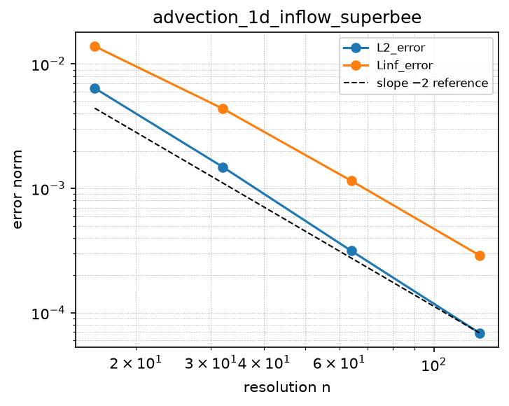
flux_limiter_superbee_D_periodic
Source: grids/cartesian_uniform_1d/rules/flux_limiter_superbee_D_periodic.esm
Rewrites ∂u/∂x at priority 10 — match pattern:
{"op": "D", "args": ["u"], "wrt": "x"}
where): fires only when u is a bare field shaped [x]. Under import-edge renaming (§9.7.7) the wrt literal and this shape follow the renamed axis together, so the rule can be imported more than once (each instance scoped to its own grid) without a first-declared-wins collision. A consumer differentiating a compound inline expression must bind it to a declared shaped observed first.Discretization — one makearray tiling the output axes; boundary conditions live in the face regions of this same rule (esm-spec §9.6.8; later regions overwrite earlier, §4.3.2):
| Region | Treatment | Value |
|---|---|---|
x ∈ [3, N−1] | interior | (u[i] + 0.5·(max(0, max(max(0, min(2·(u[i] − u[i−1]), u[i+1] − u[i])) + min(0, max(2·(u[i] − u[i−1]), u[i+1] − u[i])), max(0, min(u[i] − u[i−1], 2·(u[i+1] − u[i]))) + min(0, max(u[i] − u[i−1], 2·(u[i+1] − u[i]))))) + min(0, min(max(0, min(2·(u[i] − u[i−1]), u[i+1] − u[i])) + min(0, max(2·(u[i] − u[i−1]), u[i+1] − u[i])), max(0, min(u[i] − u[i−1], 2·(u[i+1] − u[i]))) + min(0, max(u[i] − u[i−1], 2·(u[i+1] − u[i])))))) − (u[i−1] + 0.5·(max(0, max(max(0, min(2·(u[i−1] − u[i−2]), u[i] − u[i−1])) + min(0, max(2·(u[i−1] − u[i−2]), u[i] − u[i−1])), max(0, min(u[i−1] − u[i−2], 2·(u[i] − u[i−1]))) + min(0, max(u[i−1] − u[i−2], 2·(u[i] − u[i−1]))))) + min(0, min(max(0, min(2·(u[i−1] − u[i−2]), u[i] − u[i−1])) + min(0, max(2·(u[i−1] − u[i−2]), u[i] − u[i−1])), max(0, min(u[i−1] − u[i−2], 2·(u[i] − u[i−1]))) + min(0, max(u[i−1] − u[i−2], 2·(u[i] − u[i−1])))))))) / dx for i ∈ [3, N−1] |
x = 1 | boundary face | (u[1] + 0.5·(max(0, max(max(0, min(2·(u[1] − u[N]), u[2] − u[1])) + min(0, max(2·(u[1] − u[N]), u[2] − u[1])), max(0, min(u[1] − u[N], 2·(u[2] − u[1]))) + min(0, max(u[1] − u[N], 2·(u[2] − u[1]))))) + min(0, min(max(0, min(2·(u[1] − u[N]), u[2] − u[1])) + min(0, max(2·(u[1] − u[N]), u[2] − u[1])), max(0, min(u[1] − u[N], 2·(u[2] − u[1]))) + min(0, max(u[1] − u[N], 2·(u[2] − u[1])))))) − (u[N] + 0.5·(max(0, max(max(0, min(2·(u[N] − u[N−1]), u[1] − u[N])) + min(0, max(2·(u[N] − u[N−1]), u[1] − u[N])), max(0, min(u[N] − u[N−1], 2·(u[1] − u[N]))) + min(0, max(u[N] − u[N−1], 2·(u[1] − u[N]))))) + min(0, min(max(0, min(2·(u[N] − u[N−1]), u[1] − u[N])) + min(0, max(2·(u[N] − u[N−1]), u[1] − u[N])), max(0, min(u[N] − u[N−1], 2·(u[1] − u[N]))) + min(0, max(u[N] − u[N−1], 2·(u[1] − u[N])))))))) / dx |
x = 2 | boundary face | (u[2] + 0.5·(max(0, max(max(0, min(2·(u[2] − u[1]), u[3] − u[2])) + min(0, max(2·(u[2] − u[1]), u[3] − u[2])), max(0, min(u[2] − u[1], 2·(u[3] − u[2]))) + min(0, max(u[2] − u[1], 2·(u[3] − u[2]))))) + min(0, min(max(0, min(2·(u[2] − u[1]), u[3] − u[2])) + min(0, max(2·(u[2] − u[1]), u[3] − u[2])), max(0, min(u[2] − u[1], 2·(u[3] − u[2]))) + min(0, max(u[2] − u[1], 2·(u[3] − u[2])))))) − (u[1] + 0.5·(max(0, max(max(0, min(2·(u[1] − u[N]), u[2] − u[1])) + min(0, max(2·(u[1] − u[N]), u[2] − u[1])), max(0, min(u[1] − u[N], 2·(u[2] − u[1]))) + min(0, max(u[1] − u[N], 2·(u[2] − u[1]))))) + min(0, min(max(0, min(2·(u[1] − u[N]), u[2] − u[1])) + min(0, max(2·(u[1] − u[N]), u[2] − u[1])), max(0, min(u[1] − u[N], 2·(u[2] − u[1]))) + min(0, max(u[1] − u[N], 2·(u[2] − u[1])))))))) / dx |
x = N | boundary face | (u[N] + 0.5·(max(0, max(max(0, min(2·(u[N] − u[N−1]), u[1] − u[N])) + min(0, max(2·(u[N] − u[N−1]), u[1] − u[N])), max(0, min(u[N] − u[N−1], 2·(u[1] − u[N]))) + min(0, max(u[N] − u[N−1], 2·(u[1] − u[N]))))) + min(0, min(max(0, min(2·(u[N] − u[N−1]), u[1] − u[N])) + min(0, max(2·(u[N] − u[N−1]), u[1] − u[N])), max(0, min(u[N] − u[N−1], 2·(u[1] − u[N]))) + min(0, max(u[N] − u[N−1], 2·(u[1] − u[N])))))) − (u[N−1] + 0.5·(max(0, max(max(0, min(2·(u[N−1] − u[N−2]), u[N] − u[N−1])) + min(0, max(2·(u[N−1] − u[N−2]), u[N] − u[N−1])), max(0, min(u[N−1] − u[N−2], 2·(u[N] − u[N−1]))) + min(0, max(u[N−1] − u[N−2], 2·(u[N] − u[N−1]))))) + min(0, min(max(0, min(2·(u[N−1] − u[N−2]), u[N] − u[N−1])) + min(0, max(2·(u[N−1] − u[N−2]), u[N] − u[N−1])), max(0, min(u[N−1] − u[N−2], 2·(u[N] − u[N−1]))) + min(0, max(u[N−1] − u[N−2], 2·(u[N] − u[N−1])))))))) / dx |
Second-order TVD flux-limited (superbee limiter) finite-VOLUME discretization of the advective first derivative u_x for scalar linear advection u_t = -c u_x (non-negative speed c, periodic) on cartesian_uniform_1d, in semi-discrete method-of-lines form. Structure identical to flux_limiter_minmod_D_periodic but with the superbee limiter of Roe (1986), phi(r) = max(0, min(2r, 1), min(r, 2)) — the compressive upper edge of the Sweby (1984) second-order TVD region. The consumer writes u_t = -cD(u, wrt: x); this rule emits the c-independent flux-difference D_i = (G[i+1/2] - G[i-1/2]) / dx with G[i+1/2] = u_i + 0.5phi(r_i)(u_{i+1} - u_i), r_i = (u_i - u_{i-1})/(u_{i+1} - u_i) (LeVeque 2002, eq. 6.35, semi-discrete dt->0 limit; c factors out for c > 0, +x sign baked). DIVISION-FREE GUARD: the correction 0.5phi(r_i)(u_{i+1} - u_i) is written in the algebraically-identical division-free jump form 0.5maxmod(minmod(2Dm, Dp), minmod(Dm, 2Dp)) with Dm = u_i - u_{i-1}, Dp = u_{i+1} - u_i (Roe’s double-minmod form of superbee), where minmod(a, b) = max(0, min(a, b)) + min(0, max(a, b)) and the two minmod arguments (which share sign) are combined by maxmod(p, q) = max(0, max(p, q)) + min(0, min(p, q)) — all pure max/min, no explicit division and no epsilon (verified to machine precision against phi(r)*(u_{i+1}-u_i) wherever r is defined, and finite at a zero jump). TVD, monotonicity-preserving (no new extrema; total variation non-increasing); superbee is compressive and keeps discontinuities sharp. Formally second-order where the limiter is inactive; it clips at smooth extrema, so on a periodic sin the observed order is below 2 (documented in the convergence case — L2 ~1.7, Linf ~1.2). MATCH: plain D(u, wrt: x) at priority 10, match-scoped where: {u: {shape: [x]}} (esm-spec 9.6.1); priority + shape constraint disambiguate from a sibling plain first-derivative rule and survive import-edge renaming (esm-spec 9.7.7). A model imports exactly one advection rule for x. Self-contained makearray: 4-point TVD stencil (u[i-2..i+1]); interior [3, N-1] plus the periodic-wrap faces i=1, i=2, i=N (same wrap as the minmod sibling). dx is a free name resolving to the consuming model’s spacing variable (consumer-supplied geometry contract); the periodic wrap is dx-scale-invariant.
References
- Roe, P. L. (1986). Characteristic-based schemes for the Euler equations. Ann. Rev. Fluid Mech. 18:337-365 (minmod eq. 35, superbee eq. 36).
doi:10.1146/annurev.fl.18.010186.002005 - Sweby, P. K. (1984). High resolution schemes using flux limiters for hyperbolic conservation laws. SIAM J. Numer. Anal. 21(5):995-1011.
doi:10.1137/0721062 - LeVeque, R. J. (2002). Finite Volume Methods for Hyperbolic Problems. Cambridge University Press. Section 6.11-6.12 (flux-limiter methods) and eq. (6.35); Chapter 4 (Lax-Friedrichs / Rusanov).
Conformance fixtures
- ast:
flux_limiter_superbee_D_periodic— statusactive - convergence:
advection_1d_periodic_superbee— statusactive - simulation:
advection_1d_periodic_superbee— statusactive
Convergence — case advection_1d_periodic_superbee
Error norms read from the committed golden tests/conformance/convergence/advection_1d_periodic_superbee/golden/errors.json (binding: julia; nothing recomputed for display).
| n | L2_error | observed order | Linf_error | observed order |
|---|---|---|---|---|
| 16 | 3.268e-02 | — | 4.147e-02 | — |
| 32 | 1.271e-02 | 1.36 | 2.587e-02 | 0.68 |
| 64 | 4.025e-03 | 1.66 | 1.143e-02 | 1.18 |
| 128 | 1.233e-03 | 1.71 | 4.699e-03 | 1.28 |
Expected order: 1.42 (± 0.3).
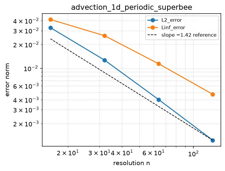
godunov_norm_D1_dirichlet_bc
Source: grids/cartesian_uniform_1d/rules/godunov_norm_D1_dirichlet_bc.esm
Rewrites √(∂u/∂x²) at priority 10 — match pattern:
{"op": "sqrt", "args": [{"op": "^", "args": [{"op": "D", "args": ["u"], "wrt": "x"}, 2]}]}
where): fires only when u is a bare field shaped [x]. Under import-edge renaming (§9.7.7) the wrt literal and this shape follow the renamed axis together, so the rule can be imported more than once (each instance scoped to its own grid) without a first-declared-wins collision. A consumer differentiating a compound inline expression must bind it to a declared shaped observed first.Discretization — one makearray tiling the output axes; boundary conditions live in the face regions of this same rule (esm-spec §9.6.8; later regions overwrite earlier, §4.3.2):
| Region | Treatment | Value |
|---|---|---|
x ∈ [2, N−1] | interior | godunov_norm_D1_interior(u)[i] = sqrt(max((u[i] − u[i−1]) / dx, 0)² + min((u[i+1] − u[i]) / dx, 0)²) for i ∈ [2, N−1] |
x = 1 | boundary face | sqrt(max((u[1] − (2·gL − u[1])) / dx, 0)² + min((u[2] − u[1]) / dx, 0)²) |
x = N | boundary face | sqrt(max((u[N] − u[N−1]) / dx, 0)² + min((2·gR − u[N] − u[N]) / dx, 0)²) |
First-order Godunov (Rouy-Tourin / Osher-Sethian) upwind discretization of the gradient magnitude |u_x| for the non-negative-speed Hamilton-Jacobi / eikonal term psi_t = -S|grad psi| (S >= 0) on cartesian_uniform_1d, with an inhomogeneous DIRICHLET (state-constraint) boundary u = g prescribed at the two walls – the natural boundary condition for eikonal / level-set problems |grad u| = f with u given on the boundary. It is the Dirichlet-closed sibling of grids/cartesian_uniform_1d/rules/godunov_norm_D1_periodic: the interior Godunov Hamiltonian and its entropy (max/min) upwind selection are UNCHANGED – only the out-of-range neighbor at the two boundary cells changes from a periodic wrap to a prescribed-value (mirror-ghost) source. COMPOUND MATCH (esm-spec 9.6.3): the rule matches the whole compound sqrt((D(u, wrt: x))^2) rooted at the outer sqrt at priority 10, IDENTICAL to godunov_norm_D1_periodic’s match, so under the outermost-first fixpoint it fires on the entire sqrt(D^2) term before any plain first-derivative rule could lower the inner D(u, wrt: x); the whole compound becomes this one makearray in a single step. Match-scoped with where {u: {shape: [x]}} (esm-spec 9.6.1) so it fires only on the gradient magnitude of a bare field over this grid’s x index set; under import-edge renaming (9.7.7) the wrt literal and the where shape follow the renamed axis. THE SCHEME: the interior [2, N-1] is a single apply_expression_template of the imported stencils/godunov_norm_D1_interior aggregate sqrt(max(D-,0)^2 + min(D+,0)^2) over the 3-point stencil. The two cell-centered walls sit half a cell outside the first and last centers, so a linear reconstruction to the wall gives the mirror ghosts u[0] = 2gL - u[1] and u[N+1] = 2gR - u[N]; substituting into the one-sided differences, the left face i=1 uses D- = (u[1] - (2gL - u[1]))/dx with D+ = (u[2] - u[1])/dx, and the right face i=N uses D+ = ((2gR - u[N]) - u[N])/dx with D- = (u[N] - u[N-1])/dx, each combined by the SAME max/min entropy norm sqrt(max(D-,0)^2 + min(D+,0)^2). gL and gR are consumer-supplied free names (the same free-name contract as the grid geometry dx; see grids/cartesian_uniform_1d/grid.esm) giving the field value at the left wall x = x0 and the right wall x = x0 + Ndx; a parameter not overridden falls back to its default (esm-spec 6: default, or 0), so gL = gR = 0 is the homogeneous case. The gL/gR terms live only in the runtime rule body, never in build-time ic/reference positions (AGENTS.md build-time scope caveat). EXACT ON A LINEAR FIELD COMPATIBLE WITH THE WALL VALUES: for u = a x + b with gL = ax0 + b and gR = a*(x0+Ndx) + b, the antisymmetric mirror ghost reproduces the true value one cell outside the wall exactly, so D- = D+ = a at BOTH boundary cells (u[1]-(2gL-u[1]) = 2(u[1]-gL) = a*dx) and the norm returns sqrt(max(a,0)^2 + min(a,0)^2) = |a| = |u_x| with no truncation error – the interior linear-exactness is preserved through the Dirichlet faces (unlike the periodic wrap, for which a non-constant ramp is a contradiction). First order O(dx) in space on smooth data; the mirror ghost is 2nd-order-consistent so the boundary retains the interior order for Dirichlet-compatible solutions. dx is a free name resolving to the consuming model’s spacing variable (consumer-supplied geometry contract). A model imports exactly one gradient-magnitude rule for x. IMPLEMENTATION NOTE: the interior Godunov Hamiltonian’s sqrt(sum of squares) is non-smooth at 0, and the min/max are non-smooth; the eikonal MMS driver problems/godunov_norm_1d_eikonal_dirichlet_mms.esm verifies this rule in Julia (Tsit5) and Python (LSODA).
References
- Osher, S., & Sethian, J. A. (1988). Fronts propagating with curvature-dependent speed: Algorithms based on Hamilton-Jacobi formulations. Journal of Computational Physics, 79(1), 12-49. The max/min upwind (entropy) construction of |grad phi| for the level-set Hamilton-Jacobi term.
doi:10.1016/0021-9991(88)90002-2 - Rouy, E., & Tourin, A. (1992). A viscosity solutions approach to shape-from-shading. SIAM Journal on Numerical Analysis, 29(3), 867-884. The Godunov Hamiltonian sqrt(max(D-,0)^2 + min(D+,0)^2) as the monotone, first-order-convergent discretization of the eikonal |grad u|.
doi:10.1137/0729053 - LeVeque, R. J. (2007). Finite Difference Methods for Ordinary and Partial Differential Equations. SIAM. Section 2.12 (cell-centered Dirichlet via mirror ghost).
Conformance fixtures
- ast:
godunov_norm_D1_dirichlet_bc— statusactive - convergence:
godunov_norm_1d_eikonal_dirichlet_mms— statusactive - simulation:
godunov_norm_1d_eikonal_dirichlet_mms— statusactive
Convergence — case godunov_norm_1d_eikonal_dirichlet_mms
Error norms read from the committed golden tests/conformance/convergence/godunov_norm_1d_eikonal_dirichlet_mms/golden/errors.json (binding: julia; nothing recomputed for display).
| n | L2_error | observed order | Linf_error | observed order |
|---|---|---|---|---|
| 16 | 9.628e-02 | — | 1.643e-01 | — |
| 32 | 6.275e-02 | 0.62 | 9.875e-02 | 0.73 |
| 64 | 2.711e-02 | 1.21 | 4.908e-02 | 1.01 |
| 128 | 1.516e-02 | 0.84 | 2.515e-02 | 0.96 |
Expected order: 1 (± 0.2).
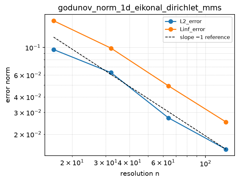
godunov_norm_D1_periodic
Source: grids/cartesian_uniform_1d/rules/godunov_norm_D1_periodic.esm
Rewrites √(∂u/∂x²) at priority 10 — match pattern:
{"op": "sqrt", "args": [{"op": "^", "args": [{"op": "D", "args": ["u"], "wrt": "x"}, 2]}]}
where): fires only when u is a bare field shaped [x]. Under import-edge renaming (§9.7.7) the wrt literal and this shape follow the renamed axis together, so the rule can be imported more than once (each instance scoped to its own grid) without a first-declared-wins collision. A consumer differentiating a compound inline expression must bind it to a declared shaped observed first.Discretization — one makearray tiling the output axes; boundary conditions live in the face regions of this same rule (esm-spec §9.6.8; later regions overwrite earlier, §4.3.2):
| Region | Treatment | Value |
|---|---|---|
x ∈ [2, N−1] | interior | sqrt(max((u[i] − u[i−1]) / dx, 0)² + min((u[i+1] − u[i]) / dx, 0)²) for i ∈ [2, N−1] |
x = 1 | boundary face | sqrt(max((u[1] − u[N]) / dx, 0)² + min((u[2] − u[1]) / dx, 0)²) |
x = N | boundary face | sqrt(max((u[N] − u[N−1]) / dx, 0)² + min((u[1] − u[N]) / dx, 0)²) |
First-order Godunov (Rouy-Tourin / Osher-Sethian) upwind discretization of the gradient magnitude |u_x| for a non-negative-speed Hamilton-Jacobi term (psi_t = -S|grad psi|, S >= 0; the level-set / eikonal norm) on cartesian_uniform_1d, with a periodic boundary. This is the 1-D reduction of the archive 2-D scheme archive/discretizations/finite_difference/godunov_norm_1st_uniform_cartesian_2d.json: where the 2-D scheme sums over axes d, the 1-D form keeps the single x term. COMPOUND MATCH (esm-spec 9.6.3 compound precedence, the canonical Godunov-Hamiltonian example cited there and in 9.6.8): the rule matches the whole compound sqrt((D(u, wrt: x))^2) rooted at the outer sqrt — cartesian’s plain-D first-derivative idiom squared under a square root, the exact structural analogue of the archive’s applies_to sqrt(grad(u,x)^2) expressed in the D convention that grids/cartesian_uniform_1d already uses (central_D1_, upwind1_D_). It carries priority 10 (>= the D2 rules’ 10) so that, under the section-9.6.3 outermost-first fixpoint, it fires on the entire sqrt(D^2) term BEFORE any plain first-derivative rule (central_D1_periodic / upwind1_D_periodic) could lower the inner D(u, wrt: x); the whole compound is replaced by this one makearray in a single step and the engine does not descend into the fresh body. Match-scoped with where: {u: {shape: [x]}} (esm-spec 9.6.1) so it fires only on the gradient magnitude of a bare field declared over this grid’s x index set; under import-edge renaming (esm-spec 9.7.7) the wrt literal and the where shape follow the renamed axis together, so two cartesian instances coexist scoped to their own grids. Because the constraint requires a bare shaped variable, a consumer forming the gradient magnitude of a COMPOUND inner expression must first bind it to a declared x-shaped observed. THE SCHEME: with backward D- = (u[i] - u[i-1]) / dx and forward D+ = (u[i+1] - u[i]) / dx, the discrete norm is sqrt( max(D-, 0)^2 + min(D+, 0)^2 ). The max/min is the entropy (upwind) fix of Osher & Sethian (1988) and Rouy & Tourin (1992): for the non-negative-speed term it selects the one-sided difference along the incoming characteristic per point (a centered difference is unstable for this hyperbolic operator). It is EXACT on a linear field: for u = a x + b the interior gives D- = D+ = a, so sqrt(max(a,0)^2 + min(a,0)^2) = |a| = |u_x| to rounding, reproducing the continuous gradient magnitude with no truncation error (the low-order analogue of the null-space property that annihilates constants, a = 0 -> 0). First order in space, O(dx), on smooth data; it retains first-order accuracy uniformly through the |grad| kinks (points where u_x changes sign) that the entropy fix is designed to resolve. Interior [2, N-1] holds the aggregate over the 3-point stencil (u[i-1], u[i], u[i+1]); the two faces i=1 and i=N are the same norm with the out-of-range neighbor wrapped PERIODICALLY (i=1 uses the ghost u[0] = u[N] in D-, i=N uses u[N+1] = u[1] in D+), so the operator is self-contained and testable on a closed circle. A periodic linear field is a contradiction (a non-zero ramp cannot wrap), so the two wrap faces carry the seam of a ramp rather than |a|; the exactness property is the interior statement, and the periodic gate that ships with this rule uses the constant/interior form (problems/godunov_norm_1d_periodic_exact.esm). dx is a free name resolving to the consuming model’s spacing variable (grids/cartesian_uniform_1d/grid.esm consumer-supplied geometry contract); the periodic wrap is dx-scale-invariant, so the rule serves any domain extent unchanged. A model imports exactly one gradient-magnitude rule for x.
References
- Osher, S., & Sethian, J. A. (1988). Fronts propagating with curvature-dependent speed: Algorithms based on Hamilton-Jacobi formulations. Journal of Computational Physics, 79(1), 12-49. The max/min upwind (entropy) construction of |grad phi| for the level-set Hamilton-Jacobi term.
doi:10.1016/0021-9991(88)90002-2 - Rouy, E., & Tourin, A. (1992). A viscosity solutions approach to shape-from-shading. SIAM Journal on Numerical Analysis, 29(3), 867-884. The Godunov Hamiltonian sqrt(max(D-,0)^2 + min(D+,0)^2) as the monotone, first-order-convergent discretization of the eikonal |grad u|.
doi:10.1137/0729053
Conformance fixtures
- ast:
godunov_norm_D1_periodic— statusactive - convergence:
godunov_norm_1d_eikonal_mms— statusactive - simulation:
godunov_norm_1d_eikonal_mms— statusactive - simulation:
godunov_norm_1d_periodic_exact— statusactive
Convergence — case godunov_norm_1d_eikonal_mms
Error norms read from the committed golden tests/conformance/convergence/godunov_norm_1d_eikonal_mms/golden/errors.json (binding: julia; nothing recomputed for display).
| n | L2_error | observed order | Linf_error | observed order |
|---|---|---|---|---|
| 16 | 2.350e-01 | — | 2.452e-01 | — |
| 32 | 1.191e-01 | 0.98 | 1.232e-01 | 0.99 |
| 64 | 6.008e-02 | 0.99 | 6.166e-02 | 1.00 |
| 128 | 3.018e-02 | 0.99 | 3.084e-02 | 1.00 |
Expected order: 1 (± 0.15).
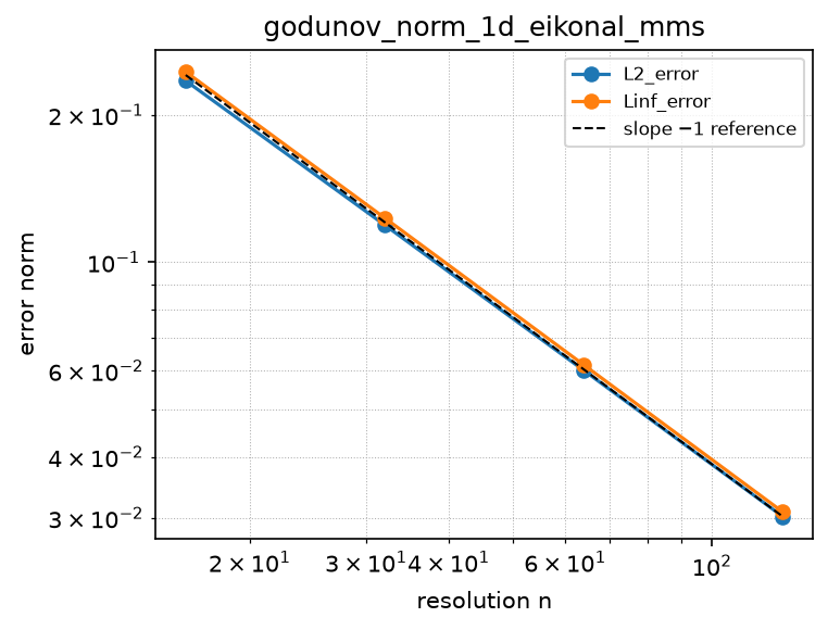
hjweno_norm_D1_dirichlet_bc
Source: grids/cartesian_uniform_1d/rules/hjweno_norm_D1_dirichlet_bc.esm
Rewrites √(∂u/∂x²) at priority 10 — match pattern:
{"op": "sqrt", "args": [{"op": "^", "args": [{"op": "D", "args": ["u"], "wrt": "x"}, 2]}]}
where): fires only when u is a bare field shaped [x]. Under import-edge renaming (§9.7.7) the wrt literal and this shape follow the renamed axis together, so the rule can be imported more than once (each instance scoped to its own grid) without a first-declared-wins collision. A consumer differentiating a compound inline expression must bind it to a declared shaped observed first.Discretization — one makearray tiling the output axes; boundary conditions live in the face regions of this same rule (esm-spec §9.6.8; later regions overwrite earlier, §4.3.2):
| Region | Treatment | Value |
|---|---|---|
x ∈ [4, N−3] | interior | hjweno_norm_D1_interior(u)[i] = sqrt(max(hjweno_recon_minus(u[i−3], u[i−2], u[i−1], u[i], u[i+1], u[i+2]), 0)² + min(hjweno_recon_plus(u[i−2], u[i−1], u[i], u[i+1], u[i+2], u[i+3]), 0)²) for i ∈ [4, N−3] |
x = 1 | boundary face | sqrt(max(hjweno_recon_minus(2·gL − u[3], 2·gL − u[2], 2·gL − u[1], u[1], u[2], u[3]), 0)² + min(hjweno_recon_plus(2·gL − u[2], 2·gL − u[1], u[1], u[2], u[3], u[4]), 0)²) |
x = 2 | boundary face | sqrt(max(hjweno_recon_minus(2·gL − u[2], 2·gL − u[1], u[1], u[2], u[3], u[4]), 0)² + min(hjweno_recon_plus(2·gL − u[1], u[1], u[2], u[3], u[4], u[5]), 0)²) |
x = 3 | boundary face | sqrt(max(hjweno_recon_minus(2·gL − u[1], u[1], u[2], u[3], u[4], u[5]), 0)² + min(hjweno_recon_plus(u[1], u[2], u[3], u[4], u[5], u[6]), 0)²) |
x = N−2 | boundary face | sqrt(max(hjweno_recon_minus(u[N−5], u[N−4], u[N−3], u[N−2], u[N−1], u[N]), 0)² + min(hjweno_recon_plus(u[N−4], u[N−3], u[N−2], u[N−1], u[N], 2·gR − u[N]), 0)²) |
x = N−1 | boundary face | sqrt(max(hjweno_recon_minus(u[N−4], u[N−3], u[N−2], u[N−1], u[N], 2·gR − u[N]), 0)² + min(hjweno_recon_plus(u[N−3], u[N−2], u[N−1], u[N], 2·gR − u[N], 2·gR − u[N−1]), 0)²) |
x = N | boundary face | sqrt(max(hjweno_recon_minus(u[N−3], u[N−2], u[N−1], u[N], 2·gR − u[N], 2·gR − u[N−1]), 0)² + min(hjweno_recon_plus(u[N−2], u[N−1], u[N], 2·gR − u[N], 2·gR − u[N−1], 2·gR − u[N−2]), 0)²) |
Fifth-order Hamilton-Jacobi WENO (Jiang-Peng 2000, WENO-Z weights) discretization of the gradient magnitude |u_x| for the non-negative-speed eikonal term psi_t = -S|grad psi| (S >= 0) on cartesian_uniform_1d, with an inhomogeneous DIRICHLET (state-constraint) boundary u = g prescribed at the two walls – the natural boundary condition for eikonal / level-set problems. It is the Dirichlet-closed sibling of grids/cartesian_uniform_1d/rules/hjweno_norm_D1_periodic and the high-order companion of godunov_norm_D1_dirichlet_bc: the interior HJ-WENO Hamiltonian |u_x| = sqrt(max(u_x^-,0)^2 + min(u_x^+,0)^2) with its fifth-order WENO-Z one-sided derivative reconstructions and its Godunov max/min entropy selection are UNCHANGED – only the out-of-range neighbors at the six near-boundary cells change from a periodic wrap to a prescribed-value (mirror-ghost) source. COMPOUND MATCH (esm-spec 9.6.3): matches the whole compound sqrt((D(u, wrt: x))^2) rooted at the outer sqrt at priority 10, IDENTICAL to the periodic and Godunov siblings, firing before any plain first-derivative rule could lower the inner D. Match-scoped with where {u: {shape: [x]}} (esm-spec 9.6.1). THE SCHEME: the interior [4, N-3] is a single apply_expression_template of the imported stencils/hjweno_norm_D1_interior aggregate (the seven-point WENO-Z reconstruction combined by the Godunov Hamiltonian). The seven-point stencil reaches i+-3, so three near-boundary cells on each side (i in {1,2,3} and {N-2,N-1,N}) are explicit makearray faces holding the SAME HJ-WENO norm with the out-of-range cells replaced by antisymmetric mirror ghosts about the prescribed wall value: for a cell-centered wall half a cell outside the first/last center, the ghost m cells outside the left wall is u[1-m] mirrored to 2gL - u[m’]= (u[0]=2gL-u[1], u[-1]=2gL-u[2], u[-2]=2gL-u[3]) and on the right u[N+1]=2gR-u[N], u[N+2]=2gR-u[N-1], u[N+3]=2gR-u[N-2]. The WENO-Z reconstruction consumes the six cell VALUES v0..v5 (it forms their divided differences internally), so each face binds the hjweno_recon_minus / hjweno_recon_plus helpers with the ghost values substituted for the out-of-range indices. gL and gR are consumer-supplied free names (same free-name contract as the grid geometry dx) giving the wall values u(x0) and u(x0+Ndx); default 0 gives the homogeneous case. The gL/gR terms live only in the runtime rule body, never in build-time ic/reference positions (AGENTS.md build-time scope caveat). EXACT ON A LINEAR FIELD COMPATIBLE WITH THE WALL VALUES: the antisymmetric mirror reflection u[1-m] = 2gL - u[m] preserves affine data to every ghost depth (2gL - u[m] equals the true value at the mirrored cell for u = a x + b with gL = a*x0 + b), so every divided difference equals a and u_x^- = u_x^+ = a at the near-boundary cells too, giving the norm |a| with no truncation error – the interior affine-exactness is preserved through the Dirichlet faces. For a manufactured g whose smooth extension is antisymmetric about the walls (e.g. sin(2 pi x) + linear, odd about every integer/half-integer in its oscillatory part), the mirror ghost reproduces the true smooth extension, so the near-boundary WENO retains the interior fifth order. Fifth order O(dx^5) in smooth regions, WENO-Z holding full order through the u_x = 0 critical points; the Godunov max/min entropy fix resolves the |grad| kinks. dx is a free name (consumer-supplied geometry contract). A model imports exactly one gradient-magnitude rule for x. IMPLEMENTATION NOTE: the HJ-WENO AST is large and its Godunov sqrt(sum of squares) / min-max is non-smooth; the eikonal MMS driver problems/hjweno_norm_1d_eikonal_dirichlet_mms.esm verifies this rule in Julia (Tsit5) and Python (LSODA); the Rust diffsol integrator lacks a step-size fail-fast guard and wedges on this stiff, non-smooth, large-AST RHS (see the case manifests’ blocked_upstream_bindings, by analogy to the periodic sibling).
References
- Jiang, G.-S., & Peng, D. (2000). Weighted ENO Schemes for Hamilton-Jacobi Equations. SIAM Journal on Scientific Computing, 21(6), 2126-2143. The HJ-WENO construction: fifth-order WENO reconstruction of the one-sided derivatives u_x^- and u_x^+ from the divided differences of u, combined by the Godunov / Osher-Sethian Hamiltonian.
doi:10.1137/S106482759732455X - Osher, S., & Sethian, J. A. (1988). Fronts propagating with curvature-dependent speed: Algorithms based on Hamilton-Jacobi formulations. Journal of Computational Physics, 79(1), 12-49. The max/min upwind (entropy) construction of |grad phi| for the level-set Hamilton-Jacobi term.
doi:10.1016/0021-9991(88)90002-2 - Rouy, E., & Tourin, A. (1992). A viscosity solutions approach to shape-from-shading. SIAM Journal on Numerical Analysis, 29(3), 867-884. The Godunov Hamiltonian sqrt(max(D-,0)^2 + min(D+,0)^2) as the monotone, first-order-convergent discretization of the eikonal |grad u|.
doi:10.1137/0729053 - Jiang, G.-S., & Shu, C.-W. (1996). Efficient Implementation of Weighted ENO Schemes. Journal of Computational Physics, 126(1), 202-228. Smoothness indicators beta_k, nonlinear weights, and the fifth-order reconstruction reused here on the one-sided divided differences.
doi:10.1006/jcph.1996.0130 - Borges, R., Carmona, M., Costa, B., & Don, W. S. (2008). An improved weighted essentially non-oscillatory scheme for hyperbolic conservation laws. Journal of Computational Physics, 227(6), 3191-3211. The WENO-Z weights that recover the full fifth order at first-order critical points (u_x = 0).
doi:10.1016/j.jcp.2007.11.038 - LeVeque, R. J. (2007). Finite Difference Methods for Ordinary and Partial Differential Equations. SIAM. Section 2.12 (cell-centered Dirichlet via mirror ghost).
Conformance fixtures
- ast:
hjweno_norm_D1_dirichlet_bc— statusactive - convergence:
hjweno_norm_1d_eikonal_dirichlet_mms— statusactive - simulation:
hjweno_norm_1d_eikonal_dirichlet_mms— statusactive
Convergence — case hjweno_norm_1d_eikonal_dirichlet_mms
Error norms read from the committed golden tests/conformance/convergence/hjweno_norm_1d_eikonal_dirichlet_mms/golden/errors.json (binding: julia; nothing recomputed for display).
| n | L2_error | observed order | Linf_error | observed order |
|---|---|---|---|---|
| 16 | 6.185e-05 | — | 9.619e-05 | — |
| 32 | 1.919e-06 | 5.01 | 3.095e-06 | 4.96 |
| 64 | 5.980e-08 | 5.00 | 1.003e-07 | 4.95 |
| 128 | 1.864e-09 | 5.00 | 3.089e-09 | 5.02 |
Expected order: 5 (± 0.3).
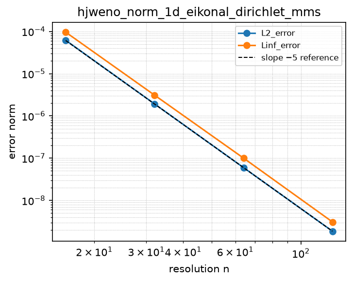
hjweno_norm_D1_periodic
Source: grids/cartesian_uniform_1d/rules/hjweno_norm_D1_periodic.esm
Rewrites √(∂u/∂x²) at priority 10 — match pattern:
{"op": "sqrt", "args": [{"op": "^", "args": [{"op": "D", "args": ["u"], "wrt": "x"}, 2]}]}
where): fires only when u is a bare field shaped [x]. Under import-edge renaming (§9.7.7) the wrt literal and this shape follow the renamed axis together, so the rule can be imported more than once (each instance scoped to its own grid) without a first-declared-wins collision. A consumer differentiating a compound inline expression must bind it to a declared shaped observed first.Discretization — one makearray tiling the output axes; boundary conditions live in the face regions of this same rule (esm-spec §9.6.8; later regions overwrite earlier, §4.3.2):
| Region | Treatment | Value |
|---|---|---|
x ∈ [4, N−3] | interior | hjweno_norm_D1_interior(u)[i] = sqrt(max(hjweno_recon_minus(u[i−3], u[i−2], u[i−1], u[i], u[i+1], u[i+2]), 0)² + min(hjweno_recon_plus(u[i−2], u[i−1], u[i], u[i+1], u[i+2], u[i+3]), 0)²) for i ∈ [4, N−3] |
x = 1 | boundary face | sqrt(max(hjweno_recon_minus(u[N−2], u[N−1], u[N], u[1], u[2], u[3]), 0)² + min(hjweno_recon_plus(u[N−1], u[N], u[1], u[2], u[3], u[4]), 0)²) |
x = 2 | boundary face | sqrt(max(hjweno_recon_minus(u[N−1], u[N], u[1], u[2], u[3], u[4]), 0)² + min(hjweno_recon_plus(u[N], u[1], u[2], u[3], u[4], u[5]), 0)²) |
x = 3 | boundary face | sqrt(max(hjweno_recon_minus(u[N], u[1], u[2], u[3], u[4], u[5]), 0)² + min(hjweno_recon_plus(u[1], u[2], u[3], u[4], u[5], u[6]), 0)²) |
x = N−2 | boundary face | sqrt(max(hjweno_recon_minus(u[N−5], u[N−4], u[N−3], u[N−2], u[N−1], u[N]), 0)² + min(hjweno_recon_plus(u[N−4], u[N−3], u[N−2], u[N−1], u[N], u[1]), 0)²) |
x = N−1 | boundary face | sqrt(max(hjweno_recon_minus(u[N−4], u[N−3], u[N−2], u[N−1], u[N], u[1]), 0)² + min(hjweno_recon_plus(u[N−3], u[N−2], u[N−1], u[N], u[1], u[2]), 0)²) |
x = N | boundary face | sqrt(max(hjweno_recon_minus(u[N−3], u[N−2], u[N−1], u[N], u[1], u[2]), 0)² + min(hjweno_recon_plus(u[N−2], u[N−1], u[N], u[1], u[2], u[3]), 0)²) |
Fifth-order Hamilton-Jacobi WENO (Jiang-Peng 2000) discretization of the gradient magnitude |u_x| for a non-negative-speed Hamilton-Jacobi term (psi_t = -S|grad psi|, S >= 0; the level-set / eikonal norm) on cartesian_uniform_1d, with a periodic boundary. It is the high-order companion of grids/cartesian_uniform_1d/rules/godunov_norm_D1_periodic: the SAME Godunov / Osher-Sethian Hamiltonian |u_x| = sqrt(max(u_x^-, 0)^2 + min(u_x^+, 0)^2), but with the first-order one-sided differences D-, D+ replaced by the fifth-order WENO-Z one-sided derivative reconstructions u_x^-, u_x^+ (see stencils/hjweno_norm_D1_interior.esm for the closed-form reconstruction, the smoothness indicators, and the WENO-Z weights). COMPOUND MATCH (esm-spec 9.6.3 compound precedence, the canonical Godunov-Hamiltonian example): the rule matches the whole compound sqrt((D(u, wrt: x))^2) rooted at the outer sqrt, IDENTICAL to godunov_norm_D1_periodic’s match, and carries the SAME priority 10, so under the section-9.6.3 outermost-first fixpoint it fires on the entire sqrt(D^2) term BEFORE any plain first-derivative rule could lower the inner D(u, wrt: x); the whole compound is replaced by this one makearray in a single step. hjweno_norm_D1_periodic and godunov_norm_D1_periodic are therefore IMPORT-SELECTED ALTERNATIVES: a consuming model imports EXACTLY ONE gradient-magnitude rule for x (the first-order Godunov for a monotone, TVD-robust scheme, or this fifth-order HJ-WENO for a smooth high-order scheme); they never compete within one document. Match-scoped with where: {u: {shape: [x]}} (esm-spec 9.6.1) so it fires only on the gradient magnitude of a bare field declared over this grid’s x index set; under import-edge renaming (esm-spec 9.7.7) the wrt literal and the where shape follow the renamed axis together, so two cartesian instances coexist scoped to their own grids. Because the constraint requires a bare shaped variable, a consumer forming the gradient magnitude of a COMPOUND inner expression must first bind it to a declared x-shaped observed. THE SCHEME (per point i): u_x^- and u_x^+ are the backward- and forward-biased WENO-Z reconstructions of the divided differences v_k = (u[m+1]-u[m])/dx (the seven-point stencil u[i-3..i+3]), and |u_x|_i = sqrt(max(u_x^-,0)^2 + min(u_x^+,0)^2). Fifth-order accurate in smooth regions (observed order 5.00 in L2 AND Linf on the smooth eikonal MMS, WENO-Z holding full order through the critical points u_x=0), entropy-satisfying at |grad| kinks (the Godunov max/min selects the incoming-characteristic branch). EXACT on a constant field (every divided difference is 0 to the bit, |u_x| = 0 exactly, the null-space property that annihilates constants) and on affine data (u_x^- = u_x^+ = a, sqrt(max(a,0)^2+min(a,0)^2) = |a|). The interior [4, N-3] holds the imported HJ-WENO aggregate; the six near-boundary cells i in {1,2,3} and {N-2,N-1,N} are explicit makearray faces holding the same Godunov-HJ-WENO norm with the out-of-range neighbors wrapped PERIODICALLY (index j<1 -> j+N, j>N -> j-N), three wrap cells on each side because the seven-point stencil reaches i+-3. The seven regions tile [1, N] exactly (N >= 7). A periodic linear field is a contradiction (a non-zero ramp cannot wrap), so the exactness property is the interior statement; the periodic gate that ships with this rule (problems/hjweno_norm_1d_periodic_exact.esm) uses the constant/interior form, and the nontrivial fifth-order accuracy is exercised on smooth data by the convergence sweep (problems/hjweno_norm_1d_eikonal_mms.esm). dx is a free name resolving to the consuming model’s spacing variable (grids/cartesian_uniform_1d/grid.esm consumer-supplied geometry contract); the periodic wrap is dx-scale-invariant, so the rule serves any domain extent unchanged. SCOPE NOTE: the 2-D companion (hjweno_norm_D2_periodic) is DEFERRED — the 2-D Godunov-HJ-WENO norm carries four one-sided WENO-Z reconstructions per cell across the nine periodic-tiling regions, giving an estimated ~15 MB lowered AST (over the ~10 MB tractability budget); the 1-D rule is the sufficient demonstration of the HJ-WENO composition (WENO reconstruction composed with the Godunov min/max Hamiltonian).
References
- Jiang, G.-S., & Peng, D. (2000). Weighted ENO Schemes for Hamilton-Jacobi Equations. SIAM Journal on Scientific Computing, 21(6), 2126-2143. The HJ-WENO construction: fifth-order WENO reconstruction of the one-sided derivatives u_x^- and u_x^+ from the divided differences of u, combined by the Godunov / Osher-Sethian Hamiltonian.
doi:10.1137/S106482759732455X - Osher, S., & Sethian, J. A. (1988). Fronts propagating with curvature-dependent speed: Algorithms based on Hamilton-Jacobi formulations. Journal of Computational Physics, 79(1), 12-49. The max/min upwind (entropy) construction of |grad phi| for the level-set Hamilton-Jacobi term.
doi:10.1016/0021-9991(88)90002-2 - Rouy, E., & Tourin, A. (1992). A viscosity solutions approach to shape-from-shading. SIAM Journal on Numerical Analysis, 29(3), 867-884. The Godunov Hamiltonian sqrt(max(D-,0)^2 + min(D+,0)^2) as the monotone discretization of the eikonal |grad u|; HJ-WENO raises the one-sided differences D-, D+ to fifth order.
doi:10.1137/0729053 - Jiang, G.-S., & Shu, C.-W. (1996). Efficient Implementation of Weighted ENO Schemes. Journal of Computational Physics, 126(1), 202-228. Smoothness indicators beta_k (eq. 2.17), nonlinear weights (eqs. 2.9-2.10), and the fifth-order reconstruction reused here on the one-sided divided differences.
doi:10.1006/jcph.1996.0130 - Borges, R., Carmona, M., Costa, B., & Don, W. S. (2008). An improved weighted essentially non-oscillatory scheme for hyperbolic conservation laws. Journal of Computational Physics, 227(6), 3191-3211. The WENO-Z weights alpha_k = d_k (1 + (tau_5/(eps+beta_k))^2) with tau_5 = |beta_0 - beta_2|, which recover the full fifth order at first-order critical points (u_x = 0) where the classic Jiang-Shu weights degrade.
doi:10.1016/j.jcp.2007.11.038 - Henrick, A. K., Aslam, T. D., & Powers, J. M. (2005). Mapped weighted essentially non-oscillatory schemes: Achieving optimal order near critical points. Journal of Computational Physics, 207(2), 542-567. The demonstration that classic WENO5 drops below fifth order at simple critical points (u_x=0, u_xx!=0), motivating the WENO-Z remedy used here.
doi:10.1016/j.jcp.2005.01.023
Conformance fixtures
- ast:
hjweno_norm_D1_periodic— statusactive - convergence:
hjweno_norm_1d_eikonal_mms— statusactive - simulation:
hjweno_norm_1d_eikonal_mms— statusactive - simulation:
hjweno_norm_1d_periodic_exact— statusactive
Convergence — case hjweno_norm_1d_eikonal_mms
Error norms read from the committed golden tests/conformance/convergence/hjweno_norm_1d_eikonal_mms/golden/errors.json (binding: julia; nothing recomputed for display).
| n | L2_error | observed order | Linf_error | observed order |
|---|---|---|---|---|
| 16 | 9.728e-05 | — | 9.652e-05 | — |
| 32 | 3.027e-06 | 5.01 | 3.046e-06 | 4.99 |
| 64 | 9.462e-08 | 5.00 | 9.542e-08 | 5.00 |
| 128 | 2.957e-09 | 5.00 | 2.984e-09 | 5.00 |
Expected order: 5 (± 0.3).
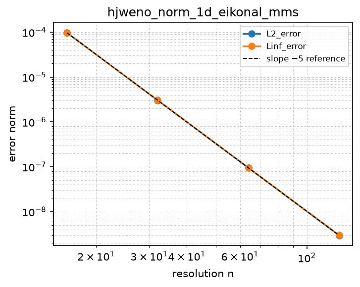
lax_friedrichs_D_inflow_bc
Source: grids/cartesian_uniform_1d/rules/lax_friedrichs_D_inflow_bc.esm
Rewrites ∂u/∂x at priority 10 — match pattern:
{"op": "D", "args": ["u"], "wrt": "x"}
where): fires only when u is a bare field shaped [x]. Under import-edge renaming (§9.7.7) the wrt literal and this shape follow the renamed axis together, so the rule can be imported more than once (each instance scoped to its own grid) without a first-declared-wins collision. A consumer differentiating a compound inline expression must bind it to a declared shaped observed first.Discretization — one makearray tiling the output axes; boundary conditions live in the face regions of this same rule (esm-spec §9.6.8; later regions overwrite earlier, §4.3.2):
| Region | Treatment | Value |
|---|---|---|
x ∈ [2, N−1] | interior | lax_friedrichs_D_interior(u)[i] = (lax_friedrichs_flux(f[i], f[i+1]) − lax_friedrichs_flux(f[i−1], f[i])) / dx for i ∈ [2, N−1] |
x = 1 | boundary face | (lax_friedrichs_flux(u[1], u[2]) − lax_friedrichs_flux(gL, u[1])) / dx |
x = N | boundary face | (lax_friedrichs_flux(u[N], u[N]) − lax_friedrichs_flux(u[N−1], u[N])) / dx |
First-order Lax-Friedrichs / Rusanov finite-volume advective first derivative u_x with OPEN boundaries – a prescribed inflow (Dirichlet) value at the upstream (left) wall and a one-sided extrapolation (outflow) closure at the downstream (right) wall – on cartesian_uniform_1d, for scalar linear advection with non-negative transport speed (a consumer writes u_t = -cD(u, wrt: x), c >= 0). This is the open-boundary sibling of rules/lax_friedrichs_D_periodic.esm and, unlike that 55-region inlined periodic file, is built THINLY on extracted stencils: the interior is a single apply of stencils/lax_friedrichs_D_interior.esm (which itself composes stencils/lax_friedrichs_flux.esm, the reusable Rusanov face flux), and the two boundary faces reuse the same flux stencil with ghost bindings – the good compositional pattern (mirroring rules/ppm_D_periodic over stencils/ppm_D_interior + ppm_flux). The semi-discrete divergence is D u[i] = (G_{i+1/2} - G_{i-1/2})/dx with G(uL,uR) = 0.5(uL+uR) - 0.5*(uR-uL). Self-contained makearray over axis x: interior [2, N-1] is the imported flux-difference; the two faces reach a ghost. INFLOW (i=1, upstream): G_{1/2} = lax_friedrichs_flux(gL, u[1]) injects the consumer-supplied inflow value gL as the left ghost, and G_{3/2} = lax_friedrichs_flux(u[1], u[2]); D u[1] = (G_{3/2} - G_{1/2})/dx. OUTFLOW (i=N, downstream): the right ghost is set by ZEROTH-ORDER EXTRAPOLATION u[N+1] = u[N], so G_{N+1/2} = lax_friedrichs_flux(u[N], u[N]), and G_{N-1/2} = lax_friedrichs_flux(u[N-1], u[N]); D u[N] = (G_{N+1/2} - G_{N-1/2})/dx. NON-REFLECTING (why extrapolation is the correct outflow closure): the Rusanov flux for a linear flux simplifies to the upwind value G(uL,uR) = uL, so G_{N+1/2} = lax_friedrichs_flux(u[N], u[N]) = u[N] regardless of the extrapolated ghost – the outflow face carries no external data and injects no spurious reflection (equivalently the extrapolation is EXACT for this flux), while G_{1/2} = lax_friedrichs_flux(gL, u[1]) = gL is exactly the prescribed inflow. So the open-boundary Lax-Friedrichs operator is bit-identical to the one-sided upwind inflow rule (upwind1_D_inflow_bc), which is why pure advection is well-posed with this single upstream wall value (a two-sided fixed-value/central closure would over-determine the outflow and need added diffusion; the one-sided upwind/LxF closure does not). gL is a free name with default 0 (the same consumer-supplied contract as rules/upwind1_D_inflow_bc’s gL and the grid geometry dx; grids/cartesian_uniform_1d/grid.esm): a consuming model declares gL as an ordinary real parameter giving the field value carried into the domain at the left wall x = x0, and an unset parameter falls back to its default (esm-spec 6; 0 = zero inflow). The gL term lives only in the runtime rule body, never in build-time ic/reference positions (AGENTS.md build-time scope caveat). dx is likewise the grid’s consumer-supplied free name; both faces are dx-scale-invariant so the rule serves any domain extent unchanged. O(dx), monotone (LxF numerical viscosity). MATCH: plain D(u, wrt: x) at priority 10 (mirroring the periodic LxF sibling), match-scoped where: {u: {shape: [x]}} (esm-spec 9.6.1) so it fires only on the first derivative of a bare field over this grid’s x index set; under import-edge renaming (esm-spec 9.7.7) the wrt literal and the where shape follow the renamed axis together, so two cartesian instances coexist. The constraint requires a bare shaped variable. A model imports exactly one advection rule for x. Sign convention: upwind for flow in +x (inflow at the left wall).
References
- LeVeque, R. J. (2002). Finite Volume Methods for Hyperbolic Problems. Cambridge University Press. Chapter 4 (Lax-Friedrichs / Rusanov); Section 7 (inflow / outflow boundary conditions for advection).
- Rusanov, V. V. (1961). Calculation of interaction of non-steady shock waves with obstacles. J. Comput. Math. Phys. USSR 1:267-279 (local Lax-Friedrichs / Rusanov flux); Lax, P. D. (1954). Weak solutions of nonlinear hyperbolic equations. Comm. Pure Appl. Math. 7:159-193.
Conformance fixtures
- ast:
lax_friedrichs_D_inflow_bc— statusactive - convergence:
advection_1d_inflow_lax_friedrichs— statusactive - simulation:
advection_1d_inflow_lax_friedrichs— statusactive
Convergence — case advection_1d_inflow_lax_friedrichs
Error norms read from the committed golden tests/conformance/convergence/advection_1d_inflow_lax_friedrichs/golden/errors.json (binding: julia; nothing recomputed for display).
| n | L2_error | observed order | Linf_error | observed order |
|---|---|---|---|---|
| 16 | 2.709e-02 | — | 2.869e-02 | — |
| 32 | 1.390e-02 | 0.96 | 1.481e-02 | 0.95 |
| 64 | 7.047e-03 | 0.98 | 7.500e-03 | 0.98 |
| 128 | 3.549e-03 | 0.99 | 3.772e-03 | 0.99 |
Expected order: 1 (± 0.2).
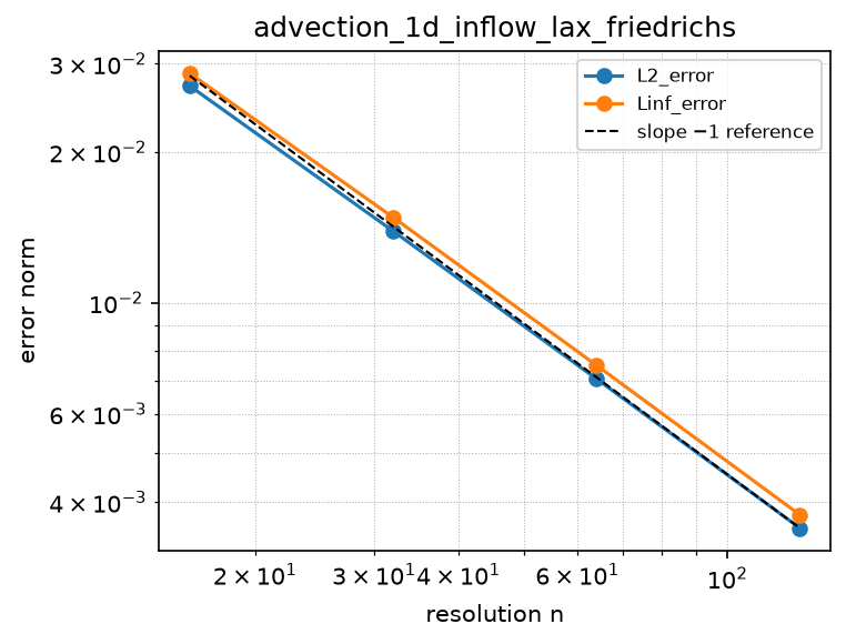
lax_friedrichs_D_periodic
Source: grids/cartesian_uniform_1d/rules/lax_friedrichs_D_periodic.esm
Rewrites ∂u/∂x at priority 10 — match pattern:
{"op": "D", "args": ["u"], "wrt": "x"}
where): fires only when u is a bare field shaped [x]. Under import-edge renaming (§9.7.7) the wrt literal and this shape follow the renamed axis together, so the rule can be imported more than once (each instance scoped to its own grid) without a first-declared-wins collision. A consumer differentiating a compound inline expression must bind it to a declared shaped observed first.Discretization — one makearray tiling the output axes; boundary conditions live in the face regions of this same rule (esm-spec §9.6.8; later regions overwrite earlier, §4.3.2):
| Region | Treatment | Value |
|---|---|---|
x ∈ [2, N−1] | interior | (0.5·(u[i] + u[i+1]) − 0.5·(u[i+1] − u[i]) − (0.5·(u[i−1] + u[i]) − 0.5·(u[i] − u[i−1]))) / dx for i ∈ [2, N−1] |
x = 1 | boundary face | (0.5·(u[1] + u[2]) − 0.5·(u[2] − u[1]) − (0.5·(u[N] + u[1]) − 0.5·(u[1] − u[N]))) / dx |
x = N | boundary face | (0.5·(u[N] + u[1]) − 0.5·(u[1] − u[N]) − (0.5·(u[N−1] + u[N]) − 0.5·(u[N] − u[N−1]))) / dx |
First-order Lax-Friedrichs / Rusanov (local Lax-Friedrichs) finite-VOLUME flux discretization of the advective first derivative u_x for the scalar linear advection u_t = -c u_x (non-negative speed c, periodic) on cartesian_uniform_1d, in semi-discrete method-of-lines form. The consumer writes u_t = -cD(u, wrt: x); this rule emits the c-independent flux-difference D_i = (G[i+1/2] - G[i-1/2]) / dx that, scaled by the consumer’s -c, gives the finite-volume tendency -(F[i+1/2] - F[i-1/2])/dx with the Lax-Friedrichs numerical flux F[i+1/2] = 0.5c*(u_i + u_{i+1}) - 0.5alpha(u_{i+1} - u_i), alpha = |c| (Rusanov). The dissipation coefficient alpha equals the SAME c the consumer multiplies by, so with c > 0 the coefficient ratio alpha/c = 1 and the flux factors as F = cG with G[i+1/2] = 0.5(u_i + u_{i+1}) - 0.5*(u_{i+1} - u_i), the c-free average-minus-dissipation form emitted here (the +x sign is baked exactly as upwind1_D_periodic bakes it; a sign-aware variant belongs in a separate rule). ALGEBRAIC NOTE: for scalar linear advection this local-LxF/Rusanov flux is exactly first-order upwind — G[i+1/2] simplifies to u_i, so D reduces to the backward difference (u_i - u_{i-1})/dx and this rule is numerically identical to upwind1_D_periodic (its convergence golden matches upwind’s to the bit). The rule is nonetheless authored in the explicit Lax-Friedrichs flux structure (central average minus |c|-scaled jump dissipation) so the migrated scheme is recognizable as its own operator; the equivalence is a genuine property of the Rusanov flux for a linear flux function, documented rather than hidden. O(dx), monotone, TVD (a maximum-principle scheme: it develops no new extrema and its total variation is non-increasing). MATCH: plain D(u, wrt: x) at priority 10, match-scoped where: {u: {shape: [x]}} (esm-spec 9.6.1) so it fires only on the first derivative of a bare field over this grid’s x index set; the priority + shape constraint disambiguate it from a sibling plain first-derivative rule (central_D1_periodic / upwind1_D_periodic) if both are ever in scope, and under import-edge renaming (esm-spec 9.7.7) the wrt literal and the where shape follow the renamed axis together. A model imports exactly one advection rule for x. Self-contained makearray: interior [2, N-1] holds the flux-difference aggregate over the 3-point stencil (u[i-1], u[i], u[i+1]); the two faces i=1 and i=N carry the same flux difference with the out-of-range neighbor wrapped PERIODICALLY (i=1 uses the ghost u[0]=u[N] in G[1/2], i=N uses u[N+1]=u[1] in G[N+1/2]). dx is a free name resolving to the consuming model’s spacing variable (grids/cartesian_uniform_1d/grid.esm consumer-supplied geometry contract); the periodic wrap is dx-scale-invariant, so the rule serves any domain extent unchanged.
References
- LeVeque, R. J. (2002). Finite Volume Methods for Hyperbolic Problems. Cambridge University Press. Section 6.11-6.12 (flux-limiter methods) and eq. (6.35); Chapter 4 (Lax-Friedrichs / Rusanov).
- Rusanov, V. V. (1961). Calculation of interaction of non-steady shock waves with obstacles. J. Comput. Math. Phys. USSR 1:267-279 (local Lax-Friedrichs / Rusanov flux); Lax, P. D. (1954). Weak solutions of nonlinear hyperbolic equations. Comm. Pure Appl. Math. 7:159-193.
Conformance fixtures
- ast:
lax_friedrichs_D_periodic— statusactive - convergence:
advection_1d_periodic_lax_friedrichs— statusactive - simulation:
advection_1d_periodic_lax_friedrichs— statusactive
Convergence — case advection_1d_periodic_lax_friedrichs
Error norms read from the committed golden tests/conformance/convergence/advection_1d_periodic_lax_friedrichs/golden/errors.json (binding: julia; nothing recomputed for display).
| n | L2_error | observed order | Linf_error | observed order |
|---|---|---|---|---|
| 16 | 1.157e-01 | — | 1.141e-01 | — |
| 32 | 5.976e-02 | 0.95 | 5.976e-02 | 0.93 |
| 64 | 3.036e-02 | 0.98 | 3.036e-02 | 0.98 |
| 128 | 1.530e-02 | 0.99 | 1.530e-02 | 0.99 |
Expected order: 1 (± 0.15).
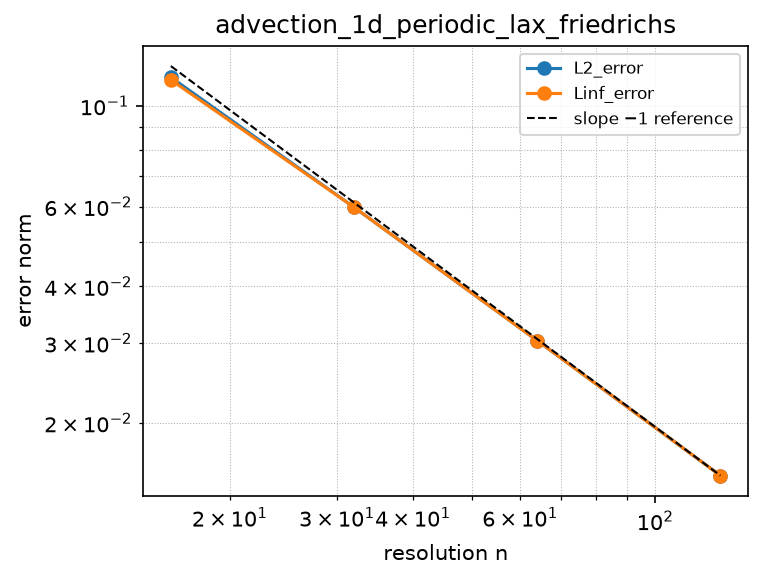
ppm_D_inflow_bc
Source: grids/cartesian_uniform_1d/rules/ppm_D_inflow_bc.esm
Rewrites ∂u/∂x at priority 10 — match pattern:
{"op": "D", "args": ["u"], "wrt": "x"}
where): fires only when u is a bare field shaped [x]. Under import-edge renaming (§9.7.7) the wrt literal and this shape follow the renamed axis together, so the rule can be imported more than once (each instance scoped to its own grid) without a first-declared-wins collision. A consumer differentiating a compound inline expression must bind it to a declared shaped observed first.Discretization — one makearray tiling the output axes; boundary conditions live in the face regions of this same rule (esm-spec §9.6.8; later regions overwrite earlier, §4.3.2):
| Region | Treatment | Value |
|---|---|---|
x ∈ [4, N−2] | interior | ppm_D_interior(u)[i] = (ppm_flux(f[i−2], f[i−1], f[i], f[i+1], f[i+2]) − ppm_flux(f[i−3], f[i−2], f[i−1], f[i], f[i+1])) / dx for i ∈ [4, N−2] |
x = 1 | boundary face | (ppm_flux(gL, gL, u[1], u[2], u[3]) − gL) / dx |
x = 2 | boundary face | (ppm_flux(gL, u[1], u[2], u[3], u[4]) − ppm_flux(gL, gL, u[1], u[2], u[3])) / dx |
x = 3 | boundary face | (ppm_flux(u[1], u[2], u[3], u[4], u[5]) − ppm_flux(gL, u[1], u[2], u[3], u[4])) / dx |
x = N−1 | boundary face | (ppm_flux(u[N−3], u[N−2], u[N−1], u[N], u[N]) − ppm_flux(u[N−4], u[N−3], u[N−2], u[N−1], u[N])) / dx |
x = N | boundary face | (ppm_flux(u[N−2], u[N−1], u[N], u[N], u[N]) − ppm_flux(u[N−3], u[N−2], u[N−1], u[N], u[N])) / dx |
Piecewise Parabolic Method (PPM; Colella & Woodward 1984) conservative finite-volume first derivative u_x on cartesian_uniform_1d with OPEN boundaries – a prescribed inflow (Dirichlet) value at the upstream (left) wall and a non-reflecting extrapolation outflow at the downstream (right) wall – for advection with non-negative transport speed (a consumer writes u_t = -c*D(u, wrt: x), c >= 0). This is the open-boundary sibling of rules/ppm_D_periodic.esm and, like it, is built THINLY on the already-well-factored PPM stencil chain rather than re-deriving any reconstruction/limiter algebra: the interior region [4, N-2] is a SINGLE apply of stencils/ppm_D_interior.esm (the conservative flux-difference aggregate D u[i] = (F_{i+1/2} - F_{i-1/2})/dx over the six-cell support u[i-3..i+2]); every boundary face reuses the SAME semi-discrete PPM upwind edge flux stencils/ppm_flux.esm (which itself composes stencils/ppm_face_value.esm eq.(1.6) 4th-order edge interpolation and stencils/ppm_limit_right.esm eqs.(1.7)-(1.10) CW84 monotonicity limiter), only with the periodic wrap of ppm_D_periodic replaced by boundary GHOST bindings – exactly the same call-site technique the periodic rule uses for its wrap cells, so no new reconstruction algebra is introduced (the ghost fill IS the boundary reconstruction, per the brief’s ‘reuse the existing PPM chain, do not duplicate it’). FLUX FORM: semi-discrete (method-of-lines) reconstructed-edge flux F_{i+1/2} = qr_lim(cell i), the CW84-limited right edge of the upwind cell, matching the periodic sibling and the ESS simulate() method-of-lines pathway (the rule supplies only the spatial operator D(u,x); the ODE integrator owns dt). The makearray tiles axis x as interior [4, N-2] plus five explicit boundary-cell faces i=1,2,3 (near the inflow wall) and i=N-1,N (near the outflow wall), mirroring the periodic rule’s five wrap faces. INFLOW WALL (left, i=1..3): the upstream cells the parabolic reconstruction needs (indices <= 0) are replaced by the prescribed inflow ghost gL (default 0), a constant upstream state. The wall face flux itself is F_{1/2} = gL – the incoming flux is the prescribed inflow value, NOT a reconstruction contaminated by downstream cells (the upwind flux at the wall must depend only on the upstream/ghost state; this matches rules/upwind1_D_inflow_bc’s (u[1]-gL)/dx face and rules/lax_friedrichs_D_inflow_bc, whose Rusanov flux reduces to gL there). The two near-wall interior faces degrade to a one-sided PPM reconstruction by filling the missing upstream ghosts with gL: F_{3/2} = ppm_flux(gL, gL, u[1], u[2], u[3]) (the CW84-limited right edge of cell 1 with its two upstream ghosts = gL) and F_{5/2} = ppm_flux(gL, u[1], u[2], u[3], u[4]) (right edge of cell 2 with one upstream ghost = gL); face F_{7/2} = ppm_flux(u[1..5]) is already fully interior and is byte-identical to the interior aggregate’s F_{i-1/2} at i=4 (shared face -> conservative). OUTFLOW WALL (right, i=N-1,N): NON-REFLECTING zeroth-order extrapolation sets the downstream ghosts u[N+1] = u[N+2] = u[N], so F_{N-1/2} = ppm_flux(u[N-3], u[N-2], u[N-1], u[N], u[N]) and F_{N+1/2} = ppm_flux(u[N-2], u[N-1], u[N], u[N], u[N]) reach only interior/self data – no external condition is imposed where characteristics leave the domain, so no spurious reflection enters and pure advection stays well-posed with the single upstream wall value (a two-sided fixed-value closure would over-determine the outflow); face F_{N-3/2} = ppm_flux(u[N-4..N]) is fully interior and byte-identical to the interior aggregate’s F_{i+1/2} at i=N-2 (shared face). CONSERVATION: every interior interface (faces 3/2 through N-1/2) is written with byte-identical ppm_flux bindings in the two cells that share it, so the divergence telescopes and mass is conserved to the bit in the interior; the domain is an OPEN system (mass enters through F_{1/2}=gL and leaves through F_{N+1/2}), so unlike the periodic ring sum(u) is not globally invariant – there is no mean-conservation claim here. ORDER (honest, to be pinned by the sweep): PPM is nominally 3rd order (parabolic) and the unlimited interior flux-difference reduces to the 4th-order central first derivative; on a SMOOTH, monotone manufactured profile (no interior extrema, e.g. cos(pi x) on [0,1]) the CW84 limiter is inactive in the interior so the interior runs near its formal order and the global observed order is set by the ONE-SIDED boundary reconstruction – sub-nominal and norm-dependent, pinned in tests/conformance/convergence/advection_1d_inflow_ppm (NOT a claim of 3rd order). Free names: gL is the consumer-supplied inflow value at the left wall x = x0 with default 0 (the same contract as rules/upwind1_D_inflow_bc’s gL and the grid geometry dx; an unset parameter falls back to its default per esm-spec 6, so gL = 0 is the zero-inflow case), appearing only in the runtime rule body, never in a build-time ic/reference position (AGENTS.md build-time scope caveat); dx is the grid’s consumer-supplied spacing (grids/cartesian_uniform_1d/grid.esm), and every boundary face is dx-scale-invariant so the rule serves any domain extent unchanged. MATCH: plain D(u, wrt: x) at priority 10 (mirroring the periodic PPM and LxF-inflow siblings) so it wins over any default-priority first-derivative rule sharing the axis; match-scoped where: {u: {shape: [x]}} (esm-spec 9.6.1) so it fires only on the first derivative of a bare field over this grid’s x index set, and under esm-spec 9.7.7 import renaming the wrt literal and the where shape follow the renamed axis together (two cartesian instances coexist). The constraint requires a bare shaped field; a consumer differentiating a compound expression must bind it to a declared x-shaped observed first. A model imports exactly one advection rule for x. Sign convention: upwind for flow in +x (inflow at the left wall); a sign-mirrored right-inflow variant belongs in a separate rule. *** MONOTONICITY UPGRADE (2026-07-13) – READ THIS. *** This rule is now genuinely BOUNDED. Its flux (../stencils/ppm_flux) previously reconstructed edges with the UNLIMITED eq. (1.7) slopes and relied on the eq. (1.10) parabola limiter alone; that combination does NOT bound the scheme. Verified in-pipeline on rules/ppm_D_periodic with sharp non-negative initial data (square / spike / sawtooth at N=32/64/128): the old chain drove a tracer in [0,1] down to -5.3e-2 and up to 1.053, i.e. it manufactured negative concentrations – not survivable in a chemistry-transport model, where they propagate into the chemistry and aerosol solvers, and where the usual fix (clip to zero) silently destroys mass conservation. The edges are now built on the CW84 eq. (1.8) MONOTONIZED slopes (../stencils/ppm_face_value_mono -> ppm_slope_mono), and the same in-pipeline test now holds the tracer EXACTLY in [0, 1] (min 0.0, max 1.0) on every profile and resolution. BOTH limiters are load-bearing and neither alone suffices: eq. (1.8) forces the interpolated EDGE to lie between the two cells it separates, while eq. (1.10)’s extremum-flattening branch is what stops outflux from a local minimum. (Independently re-derived on the stretched vertical; see grids/latlon3d/rules/ppm_D_lev_mono_noflux_bc.) ORDER CONSEQUENCES (honest): on a smooth MMS the upgrade IMPROVES the observed order for the periodic cases (1-D 1.5 -> 1.87 L2; zonal 1.64 -> 1.88 L2), because eq.(1.10)-alone clips more erratically. But where the manufactured solution has a SMOOTH INTERIOR EXTREMUM the upgrade LOWERS it: the meridional cos^4 case falls from 2.00 to 1.22 (L2), because eq. (1.8) zeroes the slope at the extremum cell and that zero also pollutes the two neighbouring edges. That is the classic 1984-limiter smooth-extremum clip, and it is the price of boundedness; the extremum-preserving Colella-Sekora (2008) limiter is the documented follow-on that would recover the order while keeping the bound. COST: the lowered AST grows ~8.5x, because ppm_limit_right must inline both edges ~5x each and a let-free AST cannot share them, so the now-larger monotonized edge is paid for ten times over; a CSE/let construct in ESM would remove this (documented follow-on). The rule’s regions, stencil support (5 cells) and boundary faces are UNCHANGED – only the edge reconstruction inside ppm_flux changed – so this is a drop-in fix, not a new operator.
References
- Colella, P., & Woodward, P. R. (1984). The Piecewise Parabolic Method (PPM) for gas-dynamical simulations. Journal of Computational Physics, 54(1), 174-201.
doi:10.1016/0021-9991(84)90143-8 - LeVeque, R. J. (2002). Finite Volume Methods for Hyperbolic Problems. Cambridge University Press. Chapter 6 (high-resolution / PPM reconstruction) and Section 7 (inflow / outflow boundary conditions for advection).
- Colella, P., & Sekora, M. D. (2008). A limiter for PPM that preserves accuracy at smooth extrema. Journal of Computational Physics, 227(15), 7069-7076.
doi:10.1016/j.jcp.2008.03.034
Conformance fixtures
- ast:
ppm_D_inflow_bc— statusactive - convergence:
advection_1d_inflow_ppm— statusactive - simulation:
advection_1d_inflow_ppm— statusactive
Convergence — case advection_1d_inflow_ppm
Error norms read from the committed golden tests/conformance/convergence/advection_1d_inflow_ppm/golden/errors.json (binding: julia; nothing recomputed for display).
| n | L2_error | observed order | Linf_error | observed order |
|---|---|---|---|---|
| 16 | 4.898e-03 | — | 9.484e-03 | — |
| 32 | 1.488e-03 | 1.72 | 3.431e-03 | 1.47 |
| 64 | 3.868e-04 | 1.94 | 8.489e-04 | 2.02 |
| 128 | 1.004e-04 | 1.95 | 2.185e-04 | 1.96 |
Expected order: 2 (± 0.2).
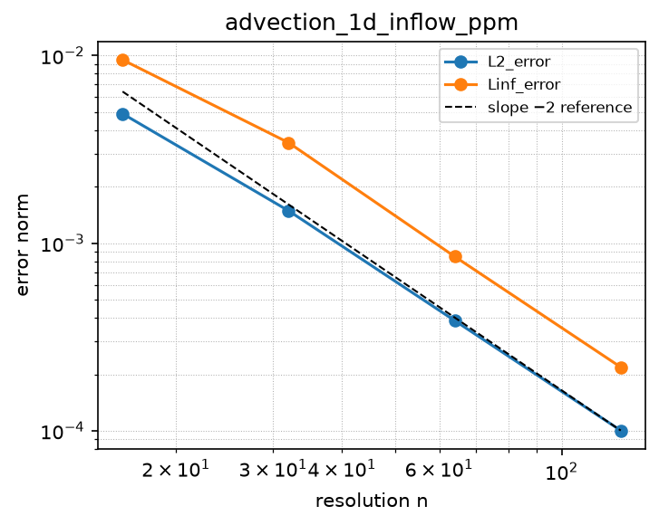
ppm_D_periodic
Source: grids/cartesian_uniform_1d/rules/ppm_D_periodic.esm
Rewrites ∂u/∂x at priority 10 — match pattern:
{"op": "D", "args": ["u"], "wrt": "x"}
where): fires only when u is a bare field shaped [x]. Under import-edge renaming (§9.7.7) the wrt literal and this shape follow the renamed axis together, so the rule can be imported more than once (each instance scoped to its own grid) without a first-declared-wins collision. A consumer differentiating a compound inline expression must bind it to a declared shaped observed first.Discretization — one makearray tiling the output axes; boundary conditions live in the face regions of this same rule (esm-spec §9.6.8; later regions overwrite earlier, §4.3.2):
| Region | Treatment | Value |
|---|---|---|
x ∈ [4, N−2] | interior | ppm_D_interior(u)[i] = (ppm_flux(f[i−2], f[i−1], f[i], f[i+1], f[i+2]) − ppm_flux(f[i−3], f[i−2], f[i−1], f[i], f[i+1])) / dx for i ∈ [4, N−2] |
x = 1 | boundary face | (ppm_flux(u[N−1], u[N], u[1], u[2], u[3]) − ppm_flux(u[N−2], u[N−1], u[N], u[1], u[2])) / dx |
x = 2 | boundary face | (ppm_flux(u[N], u[1], u[2], u[3], u[4]) − ppm_flux(u[N−1], u[N], u[1], u[2], u[3])) / dx |
x = 3 | boundary face | (ppm_flux(u[1], u[2], u[3], u[4], u[5]) − ppm_flux(u[N], u[1], u[2], u[3], u[4])) / dx |
x = N−1 | boundary face | (ppm_flux(u[N−3], u[N−2], u[N−1], u[N], u[1]) − ppm_flux(u[N−4], u[N−3], u[N−2], u[N−1], u[N])) / dx |
x = N | boundary face | (ppm_flux(u[N−2], u[N−1], u[N], u[1], u[2]) − ppm_flux(u[N−3], u[N−2], u[N−1], u[N], u[1])) / dx |
Piecewise Parabolic Method (PPM; Colella & Woodward 1984) conservative finite-volume first derivative u_x on cartesian_uniform_1d with a periodic boundary, for advection with non-negative transport speed (a consumer writes u_t = -cD(u, wrt: x), c >= 0). FLUX FORM: the SEMI-DISCRETE (method-of-lines) reconstructed-edge flux F_{i+1/2} = qr_lim(cell i), the CW84-limited right-edge value of the upwind cell – NOT the fully-discrete Courant-integral flux. The Courant form needs the CFL number nu=cdt/dx inside the operator; the ESS simulate() pathway is method-of-lines (the rule supplies only the spatial operator D(u,x) and the ODE integrator owns dt, exactly like the sibling upwind1_D_periodic / central_D1_periodic rules), so the semi-discrete edge-value flux is the composable choice and is documented as such. D u[i] = (F_{i+1/2} - F_{i-1/2})/dx; because the two adjacent cells share the identical float face flux the divergence telescopes and the periodic ring conserves sum(u) to the bit (confirmed: zero drift). RECONSTRUCTION: raw edges are CW84 eq.(1.6) 4th-order interpolation (7/12)(u_i+u_{i+1})-(1/12)(u_{i-1}+u_{i+2}); the unlimited flux-difference reduces exactly to the standard 4th-order central first derivative, so away from extrema the scheme is high order. LIMITER: CW84 eqs.(1.7)-(1.10) monotonicity limiter (stencils/ppm_limit_right, ifelse AST matching archive/discretizations/finite_volume/flux_1d_ppm.json bit-for-bit). ORDER (honest, observed): on a smooth periodic MMS the CW84 limiter still activates at the two smooth extrema (the classic clipping of the original 1984 limiter, cured only by later extremum-preserving variants), flattening the parabola there to first order; the global convergence is therefore sub-nominal and norm-dependent – about order 1.7 in L2 and 1.3 in Linf over N=16..128 (see tests/conformance/convergence/advection_1d_ppm_periodic). MONOTONICITY: the semi-discrete form is essentially non-oscillatory but NOT strictly TVD – a step develops bounded ~1.4% over/undershoot (vs ~20% unlimited); strict monotonicity would require the fully-discrete Courant-integral form, which the method-of-lines pathway cannot carry. STENCIL: the interior aggregate over [4, N-2] reads u[i-3..i+2] (6 cells); PPM needs ~3 wrap cells at the left end and ~2 at the right, so the makearray adds explicit periodic-wrap faces i=1,2,3 (left) and i=N-1,N (right), following the ESS periodic-BC face-region precedent (upwind1_D_periodic, godunov_norm_D1_periodic). Matches plain D(u, wrt: x) at priority 10 (mirroring the godunov sibling) so it wins over any default-priority first-derivative rule sharing the axis; scoped with where {u: {shape: [x]}} (esm-spec 9.6.1) so it fires only on the first derivative of a bare field over this grid’s x index set, and under 9.7.7 import renaming the wrt literal and the where shape follow the renamed axis together (two cartesian instances coexist). The constraint requires a bare shaped field; a consumer differentiating a compound expression must bind it to a declared x-shaped observed first. dx is the grid’s consumer-supplied free name (grids/cartesian_uniform_1d/grid.esm); the periodic wrap is dx-scale-invariant. *** MONOTONICITY UPGRADE (2026-07-13) – READ THIS. *** This rule is now genuinely BOUNDED. Its flux (../stencils/ppm_flux) previously reconstructed edges with the UNLIMITED eq. (1.7) slopes and relied on the eq. (1.10) parabola limiter alone; that combination does NOT bound the scheme. Verified in-pipeline on rules/ppm_D_periodic with sharp non-negative initial data (square / spike / sawtooth at N=32/64/128): the old chain drove a tracer in [0,1] down to -5.3e-2 and up to 1.053, i.e. it manufactured negative concentrations – not survivable in a chemistry-transport model, where they propagate into the chemistry and aerosol solvers, and where the usual fix (clip to zero) silently destroys mass conservation. The edges are now built on the CW84 eq. (1.8) MONOTONIZED slopes (../stencils/ppm_face_value_mono -> ppm_slope_mono), and the same in-pipeline test now holds the tracer EXACTLY in [0, 1] (min 0.0, max 1.0) on every profile and resolution. BOTH limiters are load-bearing and neither alone suffices: eq. (1.8) forces the interpolated EDGE to lie between the two cells it separates, while eq. (1.10)’s extremum-flattening branch is what stops outflux from a local minimum. (Independently re-derived on the stretched vertical; see grids/latlon3d/rules/ppm_D_lev_mono_noflux_bc.) ORDER CONSEQUENCES (honest): on a smooth MMS the upgrade IMPROVES the observed order for the periodic cases (1-D 1.5 -> 1.87 L2; zonal 1.64 -> 1.88 L2), because eq.(1.10)-alone clips more erratically. But where the manufactured solution has a SMOOTH INTERIOR EXTREMUM the upgrade LOWERS it: the meridional cos^4 case falls from 2.00 to 1.22 (L2), because eq. (1.8) zeroes the slope at the extremum cell and that zero also pollutes the two neighbouring edges. That is the classic 1984-limiter smooth-extremum clip, and it is the price of boundedness; the extremum-preserving Colella-Sekora (2008) limiter is the documented follow-on that would recover the order while keeping the bound. COST: the lowered AST grows ~8.5x, because ppm_limit_right must inline both edges ~5x each and a let-free AST cannot share them, so the now-larger monotonized edge is paid for ten times over; a CSE/let construct in ESM would remove this (documented follow-on). The rule’s regions, stencil support (5 cells) and boundary faces are UNCHANGED – only the edge reconstruction inside ppm_flux changed – so this is a drop-in fix, not a new operator.
References
- Colella, P., & Woodward, P. R. (1984). The Piecewise Parabolic Method (PPM) for gas-dynamical simulations. Journal of Computational Physics, 54(1), 174-201.
doi:10.1016/0021-9991(84)90143-8 - Lin, S.-J., & Rood, R. B. (1996). Multidimensional flux-form semi-Lagrangian transport schemes. Monthly Weather Review, 124(9), 2046-2070. Flux-form finite-volume advection composition.
doi:10.1175/1520-0493(1996)124<2046:MFFSLT>2.0.CO;2 - Colella, P., & Sekora, M. D. (2008). A limiter for PPM that preserves accuracy at smooth extrema. Journal of Computational Physics, 227(15), 7069-7076.
doi:10.1016/j.jcp.2008.03.034
Conformance fixtures
- ast:
ppm_D_periodic— statusactive - convergence:
advection_1d_ppm_periodic— statusactive - simulation:
advection_1d_ppm_periodic— statusactive
Convergence — case advection_1d_ppm_periodic
Error norms read from the committed golden tests/conformance/convergence/advection_1d_ppm_periodic/golden/errors.json (binding: julia; nothing recomputed for display).
| n | L2_error | observed order | Linf_error | observed order |
|---|---|---|---|---|
| 16 | 2.631e-02 | — | 3.333e-02 | — |
| 32 | 7.888e-03 | 1.74 | 1.405e-02 | 1.25 |
| 64 | 2.155e-03 | 1.87 | 5.051e-03 | 1.48 |
| 128 | 5.739e-04 | 1.91 | 1.706e-03 | 1.57 |
Expected order: 1.68 (± 0.3).
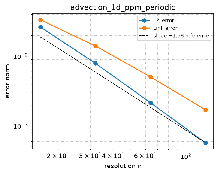
upwind1_D_inflow_bc
Source: grids/cartesian_uniform_1d/rules/upwind1_D_inflow_bc.esm
Rewrites ∂f/∂x — match pattern:
{"op": "D", "args": ["f"], "wrt": "x"}
where): fires only when f is a bare field shaped [x]. Under import-edge renaming (§9.7.7) the wrt literal and this shape follow the renamed axis together, so the rule can be imported more than once (each instance scoped to its own grid) without a first-declared-wins collision. A consumer differentiating a compound inline expression must bind it to a declared shaped observed first.Discretization — one makearray tiling the output axes; boundary conditions live in the face regions of this same rule (esm-spec §9.6.8; later regions overwrite earlier, §4.3.2):
| Region | Treatment | Value |
|---|---|---|
x ∈ [2, N] | interior | upwind1_D_interior(f)[i] = (f[i] − f[i−1]) / dx for i ∈ [2, N] |
x = 1 | boundary face | (f[1] − gL) / dx |
First-order upwind (backward) first derivative with a prescribed inflow (Dirichlet) boundary at the left wall on cartesian_uniform_1d, for advection with non-negative transport speed. Interior [2, N]: the imported backward stencil (f[i] - f[i-1])/dx. The i=N (right, outflow) cell needs no boundary closure — the backward stencil already reaches only interior/self points, which is exactly the upwind bias for flow in +x — so it is covered by the interior region. Only the i=1 (left, inflow) cell needs a wall value: face i=1 = (f[1] - gL)/dx, where the ghost half a cell outside the first center is replaced by the consumer-supplied inflow value gL. gL is a free name (the same consumer-supplied contract as the grid geometry dx and as rules/central_D2_dirichlet_bc’s gL/gR wall values; see grids/cartesian_uniform_1d/grid.esm): a consuming model declares gL as an ordinary real parameter giving the field value carried into the domain at the left wall x = x0, and a parameter left unset falls back to its default (esm-spec 6; default, or 0), so gL = 0 is the zero-inflow case. The gL term lives only in the runtime rule body, never in build-time ic/reference positions (AGENTS.md build-time scope caveat). dx is likewise a free name resolving to the consuming model’s spacing (the grid’s consumer-supplied geometry contract) — the inflow face is dx-scale-invariant, so the rule serves any domain extent unchanged. Matches plain D(f, wrt: x) at default priority, so compound rules fire first, match-scoped with where: {f: {shape: [x]}} (esm-spec 9.6.1) so it fires only on the first derivative of a bare field declared over this grid’s x index set; under import-edge renaming (esm-spec 9.7.7) the wrt literal and the where shape follow the renamed axis together, so two cartesian instances coexist scoped to their own grids. The constraint requires a bare shaped variable. O(dx). Sign convention: upwind for flow in +x (inflow at the left wall); a sign-aware or right-inflow variant belongs in a separate rule. A model imports exactly one first-derivative rule for x, never more than one.
References
- LeVeque, R. J. (2002). Finite Volume Methods for Hyperbolic Problems. Cambridge University Press. Section 4.8 (upwind methods) and Section 7 (inflow boundary conditions for advection).
Conformance fixtures
- ast:
upwind1_D_inflow_bc— statusactive - convergence:
advection_1d_inflow_upwind— statusactive - simulation:
advection_1d_inflow_upwind— statusactive
Convergence — case advection_1d_inflow_upwind
Error norms read from the committed golden tests/conformance/convergence/advection_1d_inflow_upwind/golden/errors.json (binding: julia; nothing recomputed for display).
| n | L2_error | observed order | Linf_error | observed order |
|---|---|---|---|---|
| 16 | 2.709e-02 | — | 2.869e-02 | — |
| 32 | 1.390e-02 | 0.96 | 1.481e-02 | 0.95 |
| 64 | 7.047e-03 | 0.98 | 7.500e-03 | 0.98 |
| 128 | 3.549e-03 | 0.99 | 3.772e-03 | 0.99 |
Expected order: 1 (± 0.2).
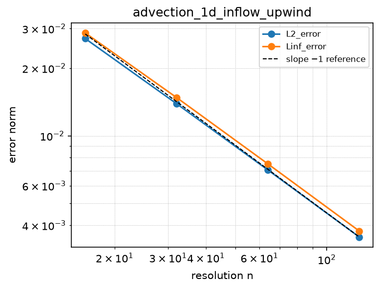
upwind1_D_inflow_right_bc
Source: grids/cartesian_uniform_1d/rules/upwind1_D_inflow_right_bc.esm
Rewrites ∂f/∂x — match pattern:
{"op": "D", "args": ["f"], "wrt": "x"}
where): fires only when f is a bare field shaped [x]. Under import-edge renaming (§9.7.7) the wrt literal and this shape follow the renamed axis together, so the rule can be imported more than once (each instance scoped to its own grid) without a first-declared-wins collision. A consumer differentiating a compound inline expression must bind it to a declared shaped observed first.Discretization — one makearray tiling the output axes; boundary conditions live in the face regions of this same rule (esm-spec §9.6.8; later regions overwrite earlier, §4.3.2):
| Region | Treatment | Value |
|---|---|---|
x ∈ [1, N−1] | interior | upwind1_D_forward_interior(f)[i] = (f[i+1] − f[i]) / dx for i ∈ [1, N−1] |
x = N | boundary face | (gR − f[N]) / dx |
First-order upwind (FORWARD) first derivative with a prescribed inflow (Dirichlet) boundary at the RIGHT wall on cartesian_uniform_1d, for advection with non-positive transport speed (flow in -x). This is the sign-mirror of rules/upwind1_D_inflow_bc.esm (which handles flow in +x with a left inflow); its own description notes that ‘a sign-aware or right-inflow variant belongs in a separate rule’ – this is that variant. Interior [1, N-1]: the imported forward stencil (f[i+1] - f[i])/dx (stencils/upwind1_D_forward_interior.esm). The i=1 (left, OUTFLOW) cell needs no boundary closure – the forward stencil reaches only interior/self points (f[1], f[2]), which is exactly the upwind bias for flow in -x, so it is covered by the interior region. Only the i=N (right, INFLOW) cell needs a wall value: face i=N = (gR - f[N])/dx, where the ghost f[N+1] half a cell outside the last center is replaced by the consumer-supplied inflow value gR. gR is a free name (the same consumer-supplied contract as the grid geometry dx and as rules/upwind1_D_inflow_bc’s gL / rules/central_D2_dirichlet_bc’s gL/gR wall values; see grids/cartesian_uniform_1d/grid.esm): a consuming model declares gR as an ordinary real parameter giving the field value carried into the domain at the right wall x = x0 + N*dx, and a parameter left unset falls back to its default (esm-spec 6; default, or 0), so gR = 0 is the zero-inflow case. The gR term lives only in the runtime rule body, never in build-time ic/reference positions (AGENTS.md build-time scope caveat). dx is likewise a free name resolving to the consuming model’s spacing (the grid’s consumer-supplied geometry contract) – the inflow face is dx-scale-invariant, so the rule serves any domain extent unchanged. NON-REFLECTING WELL-POSEDNESS: like its left-inflow mirror this is a one-sided (upwind) closure – the inflow face injects the prescribed upstream value and the outflow (left) face uses only interior data, so no external condition is imposed where characteristics leave the domain. Pure advection is therefore well-posed with this single wall value (a two-sided fixed-value/central closure would over-determine the outflow and need added diffusion; the one-sided upwind closure does not). Matches plain D(f, wrt: x) at default priority, so compound rules fire first, match-scoped with where: {f: {shape: [x]}} (esm-spec 9.6.1) so it fires only on the first derivative of a bare field declared over this grid’s x index set; under import-edge renaming (esm-spec 9.7.7) the wrt literal and the where shape follow the renamed axis together, so two cartesian instances coexist scoped to their own grids. The constraint requires a bare shaped variable. O(dx). Sign convention: upwind for flow in -x (inflow at the right wall); the +x / left-inflow variant is rules/upwind1_D_inflow_bc.esm. A model imports exactly one first-derivative rule for x, never more than one.
References
- LeVeque, R. J. (2002). Finite Volume Methods for Hyperbolic Problems. Cambridge University Press. Section 4.8 (upwind methods) and Section 7 (inflow boundary conditions for advection).
Conformance fixtures
- ast:
upwind1_D_inflow_right_bc— statusactive - convergence:
advection_1d_inflow_right_upwind— statusactive - simulation:
advection_1d_inflow_right_upwind— statusactive
Convergence — case advection_1d_inflow_right_upwind
Error norms read from the committed golden tests/conformance/convergence/advection_1d_inflow_right_upwind/golden/errors.json (binding: julia; nothing recomputed for display).
| n | L2_error | observed order | Linf_error | observed order |
|---|---|---|---|---|
| 16 | 2.709e-02 | — | 2.869e-02 | — |
| 32 | 1.390e-02 | 0.96 | 1.481e-02 | 0.95 |
| 64 | 7.047e-03 | 0.98 | 7.500e-03 | 0.98 |
| 128 | 3.549e-03 | 0.99 | 3.772e-03 | 0.99 |
Expected order: 1 (± 0.2).
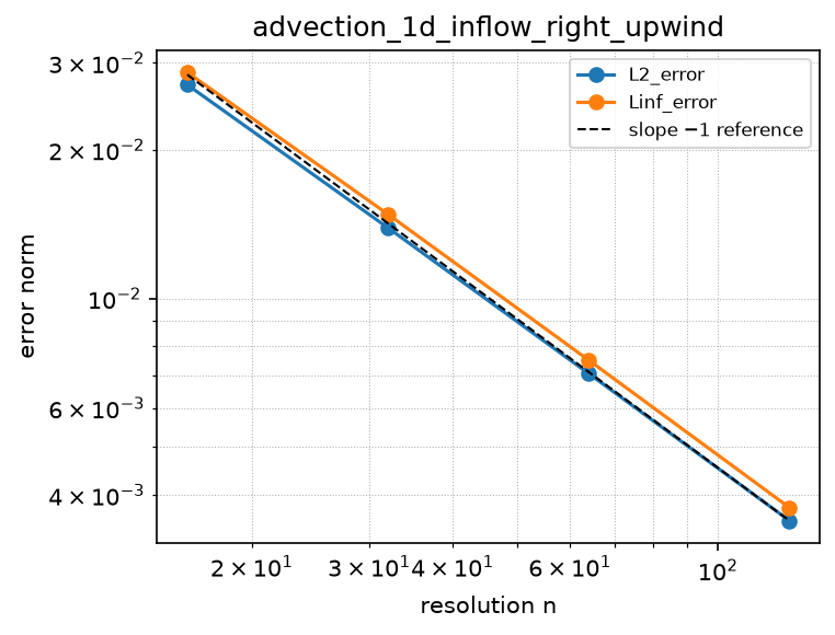
upwind1_D_periodic
Source: grids/cartesian_uniform_1d/rules/upwind1_D_periodic.esm
Rewrites ∂f/∂x — match pattern:
{"op": "D", "args": ["f"], "wrt": "x"}
where): fires only when f is a bare field shaped [x]. Under import-edge renaming (§9.7.7) the wrt literal and this shape follow the renamed axis together, so the rule can be imported more than once (each instance scoped to its own grid) without a first-declared-wins collision. A consumer differentiating a compound inline expression must bind it to a declared shaped observed first.Discretization — one makearray tiling the output axes; boundary conditions live in the face regions of this same rule (esm-spec §9.6.8; later regions overwrite earlier, §4.3.2):
| Region | Treatment | Value |
|---|---|---|
x ∈ [2, N] | interior | upwind1_D_interior(f)[i] = (f[i] − f[i−1]) / dx for i ∈ [2, N] |
x = 1 | boundary face | (f[1] − f[N]) / dx |
First-order upwind (backward) first derivative with periodic boundary on cartesian_uniform_1d, for advection with non-negative transport speed: interior i in [2, N]: (f[i] - f[i-1]) / dx; the i=1 face wraps periodically to (f[1] - f[N]) / dx. The wrap is an explicit makearray face region, following the ESS pde_simulation fixture precedent for periodic boundaries. dx is a free name resolving to the consuming model’s spacing variable (the grid’s consumer-supplied geometry contract; see grids/cartesian_uniform_1d/grid.esm) — the periodic wrap itself is dx-scale-invariant, so the rule serves any domain extent unchanged. Matches plain D(f, wrt: x) at default priority, so compound rules (e.g. a second-derivative rule at priority 10) fire first, match-scoped with where: {f: {shape: [x]}} (esm-spec 9.6.1) so it fires only on the first derivative of a bare field declared over this grid’s x index set (not on any unrelated D(., wrt: x) reusing the axis name); under import-edge renaming (esm-spec 9.7.7) the wrt literal and the where shape follow the renamed axis together, so two cartesian instances coexist scoped to their own grids. The constraint requires a bare shaped variable. O(dx). Sign convention: upwind for flow in +x; a sign-aware variant belongs in a separate rule.
References
- LeVeque, R. J. (2002). Finite Volume Methods for Hyperbolic Problems. Cambridge University Press. Section 4.8 (upwind methods).
Conformance fixtures
- ast:
upwind1_D_periodic— statusactive - convergence:
advection_1d_periodic— statusactive - simulation:
advection_1d_periodic— statusactive
Convergence — case advection_1d_periodic
Error norms read from the committed golden tests/conformance/convergence/advection_1d_periodic/golden/errors.json (binding: julia; nothing recomputed for display).
| n | L2_error | observed order | Linf_error | observed order |
|---|---|---|---|---|
| 16 | 1.157e-01 | — | 1.141e-01 | — |
| 32 | 5.976e-02 | 0.95 | 5.976e-02 | 0.93 |
| 64 | 3.036e-02 | 0.98 | 3.036e-02 | 0.98 |
| 128 | 1.530e-02 | 0.99 | 1.530e-02 | 0.99 |
Expected order: 1 (± 0.15).
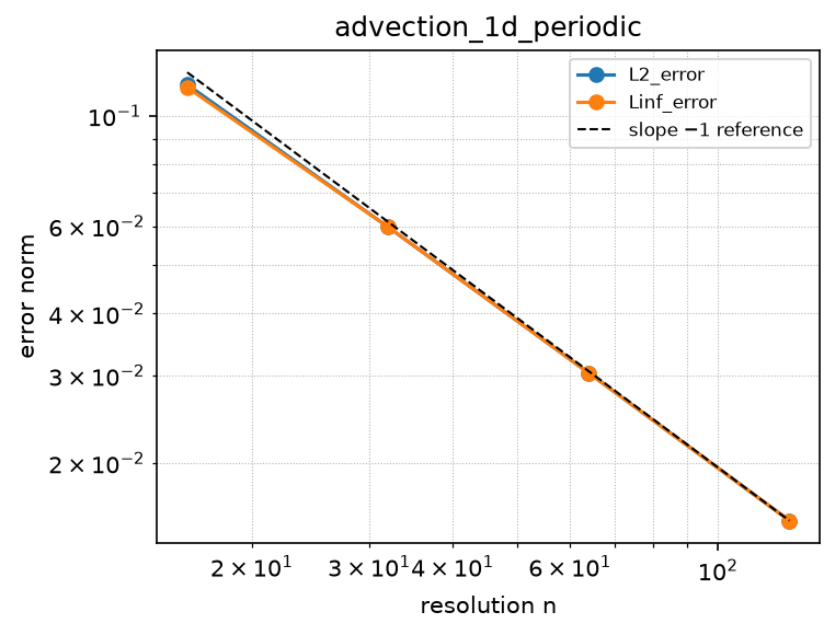
varcoeff_laplacian_dirichlet_bc
Source: grids/cartesian_uniform_1d/rules/varcoeff_laplacian_dirichlet_bc.esm
Rewrites ∂(k·∂u/∂x)/∂x at priority 10 — match pattern:
{"op": "D", "args": [{"op": "*", "args": ["k", {"op": "D", "args": ["u"], "wrt": "x"}]}], "wrt": "x"}
where): fires only when u is a bare field shaped [x]; k is a bare field shaped [x]. Under import-edge renaming (§9.7.7) the wrt literal and this shape follow the renamed axis together, so the rule can be imported more than once (each instance scoped to its own grid) without a first-declared-wins collision. A consumer differentiating a compound inline expression must bind it to a declared shaped observed first.Discretization — one makearray tiling the output axes; boundary conditions live in the face regions of this same rule (esm-spec §9.6.8; later regions overwrite earlier, §4.3.2):
| Region | Treatment | Value |
|---|---|---|
x ∈ [2, N−1] | interior | varcoeff_laplacian_interior(u, k)[i] = ((0.5·(k[i] + k[i+1]))·(u[i+1] − u[i]) − (0.5·(k[i−1] + k[i]))·(u[i] − u[i−1])) / dx² for i ∈ [2, N−1] |
x = 1 | boundary face | ((0.5·(k[1] + k[2]))·(u[2] − u[1]) − (2·k[1])·(u[1] − gL)) / dx² |
x = N | boundary face | ((0.5·(k[N−1] + k[N]))·(u[N−1] − u[N]) + (2·k[N])·(gR − u[N])) / dx² |
Conservative finite-volume VARIABLE-COEFFICIENT / NONLINEAR Laplacian div(k grad u) with inhomogeneous DIRICHLET (fixed-value) boundaries on cartesian_uniform_1d, cell-centered. The operator carries a coefficient, so a bare laplacian match cannot express it; the rule matches the CONSERVATIVE COMPOUND the consumer writes, D( {op:, args:[k, D(u,wrt:x)]}, wrt:x ) – outer-D of (k times the inner spatial gradient) – at priority 10, so under esm-spec 9.6.3 outermost-first compound precedence it fires on the whole compound before any plain-D rule could lower the inner derivative. BOTH operands are match wildcards bound to consumer fields: u (the state, inner D’s argument) and k (the coefficient, the LEFT factor of the product); matching is structural and non-commutative, so the consumer MUST write the coefficient on the LEFT: k * D(u, wrt:x). Match-scoped with where {u:{shape:[x]}, k:{shape:[x]}} (esm-spec 9.6.1) so it fires only on this grid’s declared x-shaped fields; under import-edge renaming (esm-spec 9.7.7) the wrt literals and both where shapes follow the renamed axis together. ONE rule serves the VARIABLE-COEFFICIENT case (k=k(x), a given field) and the NONLINEAR case (k declared as an observed k=f(u)); the body only reads k by index at the faces, so a state-dependent k just makes the expanded stencil nonlinear in u with no reformulation. AUTHORING CONTRACT for k (identical to varcoeff_laplacian_zero_flux_bc): k is a declared x-shaped field; an aggregate-observed coefficient MUST loop over an index DISTINCT from the stencil’s interior index i (the library convention is gi), because it is inlined into the stencil’s [2,N-1] aggregate and a shared loop-index name is captured. Face conductivity is the ARITHMETIC MEAN kf[i+1/2]=(k[i]+k[i+1])/2 (O(dx^2) at the face for a differentiable coefficient, affine in k so it composes with the nonlinear dual). Interior [2, N-1]: the imported conservative flux-difference stencil. Faces i=1 and i=N: mirror-ghost elimination against a prescribed wall value combined with the boundary-face conductivity. On this cell-centered grid the wall sits half a cell outside the first/last center, so linear reconstruction to the wall gives u[0]=2gL-u[1] (and u[N+1]=2gR-u[N]); the left domain-face flux F[1/2]=kf[1/2](u[1]-u[0])/dx uses the wall conductivity k[1] (the arithmetic-mean face value degenerates to the first cell value under the even ghost k[0]=k[1]), so F[1/2]=k[1]2(u[1]-gL)/dx and L u[1] = ( (k[1]+k[2])/2 (u[2]-u[1]) - 2 k[1] (u[1]-gL) ) / dx^2; symmetrically at the right wall F[N+1/2]=k[N]2(gR-u[N])/dx and L u[N] = ( (k[N-1]+k[N])/2 (u[N-1]-u[N]) + 2 k[N] (gR-u[N]) ) / dx^2. gL and gR are consumer-supplied free names (the same free-name contract as the grid geometry dx; see grids/cartesian_uniform_1d/grid.esm) giving the field value at the left wall x=x0 and the right wall x=x0+N*dx; a consuming model declares them as ordinary real parameters, and a parameter not overridden falls back to its default (esm-spec 6: default, or 0), so gL=gR=0 is the homogeneous-Dirichlet case. The gL/gR terms live only in the runtime rule body, never in build-time ic/reference positions (AGENTS.md build-time scope caveat). Reduces to central_D2_dirichlet_bc when k is spatially constant (k[1]=k[N]=1 gives the mirror-ghost residuals (u[2]-3u[1]+2gL)/dx^2 and (u[N-1]-3u[N]+2gR)/dx^2), and to varcoeff_laplacian_zero_flux_bc’s interior stencil in [2,N-1]. Interior O(dx^2); the one-sided mirror-ghost faces are O(dx) locally, preserving global 2nd-order L2 convergence for Dirichlet-compatible solutions. A model imports exactly one second-derivative/Laplacian rule for x.
References
- LeVeque, R. J. (2007). Finite Difference Methods for Ordinary and Partial Differential Equations. SIAM. Section 2.15 (variable-coefficient conservative form) and Section 2.12 (cell-centered Dirichlet via mirror ghost).
Conformance fixtures
- ast:
varcoeff_laplacian_dirichlet_bc— statusactive - convergence:
heat_1d_varcoeff_dirichlet— statusactive - simulation:
heat_1d_varcoeff_dirichlet— statusactive
Convergence — case heat_1d_varcoeff_dirichlet
Error norms read from the committed golden tests/conformance/convergence/heat_1d_varcoeff_dirichlet/golden/errors.json (binding: julia; nothing recomputed for display).
| n | L2_error | observed order | Linf_error | observed order |
|---|---|---|---|---|
| 16 | 2.366e-04 | — | 2.108e-04 | — |
| 32 | 5.687e-05 | 2.06 | 5.193e-05 | 2.02 |
| 64 | 1.408e-05 | 2.01 | 1.290e-05 | 2.01 |
| 128 | 3.513e-06 | 2.00 | 3.218e-06 | 2.00 |
Expected order: 2 (± 0.2).
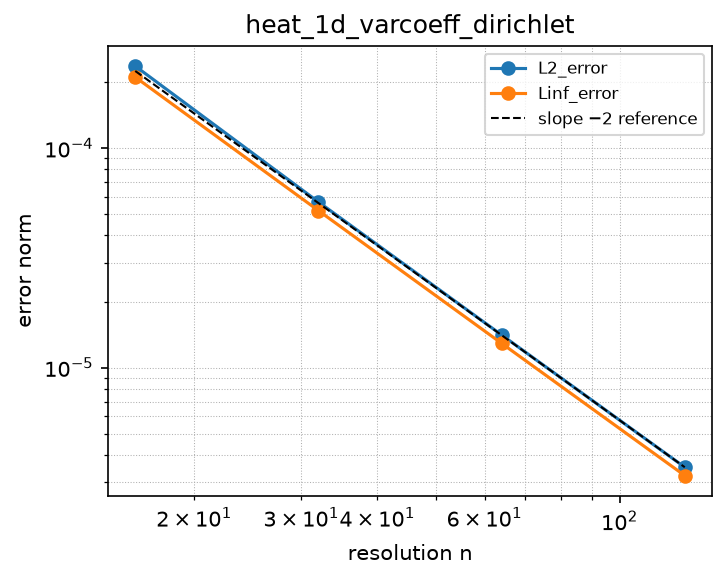
varcoeff_laplacian_neumann_bc
Source: grids/cartesian_uniform_1d/rules/varcoeff_laplacian_neumann_bc.esm
Rewrites ∂(k·∂u/∂x)/∂x at priority 10 — match pattern:
{"op": "D", "args": [{"op": "*", "args": ["k", {"op": "D", "args": ["u"], "wrt": "x"}]}], "wrt": "x"}
where): fires only when u is a bare field shaped [x]; k is a bare field shaped [x]. Under import-edge renaming (§9.7.7) the wrt literal and this shape follow the renamed axis together, so the rule can be imported more than once (each instance scoped to its own grid) without a first-declared-wins collision. A consumer differentiating a compound inline expression must bind it to a declared shaped observed first.Discretization — one makearray tiling the output axes; boundary conditions live in the face regions of this same rule (esm-spec §9.6.8; later regions overwrite earlier, §4.3.2):
| Region | Treatment | Value |
|---|---|---|
x ∈ [2, N−1] | interior | varcoeff_laplacian_interior(u, k)[i] = ((0.5·(k[i] + k[i+1]))·(u[i+1] − u[i]) − (0.5·(k[i−1] + k[i]))·(u[i] − u[i−1])) / dx² for i ∈ [2, N−1] |
x = 1 | boundary face | ((0.5·(k[1] + k[2]))·(u[2] − u[1])) / dx² − qL/dx |
x = N | boundary face | ((0.5·(k[N−1] + k[N]))·(u[N−1] − u[N])) / dx² + qR/dx |
Conservative finite-volume VARIABLE-COEFFICIENT / NONLINEAR Laplacian div(k grad u) with inhomogeneous NEUMANN (fixed-flux) boundaries on cartesian_uniform_1d, cell-centered. The operator carries a coefficient, so a bare laplacian match cannot express it; the rule matches the CONSERVATIVE COMPOUND the consumer writes, D( {op:, args:[k, D(u,wrt:x)]}, wrt:x ) – outer-D of (k times the inner spatial gradient) – at priority 10, so under esm-spec 9.6.3 outermost-first compound precedence it fires on the whole compound before any plain-D rule could lower the inner derivative. BOTH operands are match wildcards bound to consumer fields: u (the state, inner D’s argument) and k (the coefficient, the LEFT factor of the product); matching is structural and non-commutative, so the consumer MUST write the coefficient on the LEFT: k * D(u, wrt:x). Match-scoped with where {u:{shape:[x]}, k:{shape:[x]}} (esm-spec 9.6.1) so it fires only on this grid’s declared x-shaped fields; under import-edge renaming (esm-spec 9.7.7) the wrt literals and both where shapes follow the renamed axis together. ONE rule serves the VARIABLE-COEFFICIENT case (k=k(x), a given field) and the NONLINEAR case (k declared as an observed k=f(u)); the body only reads k by index at the faces, so a state-dependent k just makes the expanded stencil nonlinear in u with no reformulation. AUTHORING CONTRACT for k (identical to varcoeff_laplacian_zero_flux_bc): k is a declared x-shaped field; an aggregate-observed coefficient MUST loop over an index DISTINCT from the stencil’s interior index i (the library convention is gi), because it is inlined into the stencil’s [2,N-1] aggregate and a shared loop-index name is captured. Face conductivity is the ARITHMETIC MEAN kf[i+1/2]=(k[i]+k[i+1])/2. Interior [2, N-1]: the imported conservative flux-difference stencil. Faces i=1 and i=N: the domain-boundary face flux is PRESCRIBED DIRECTLY – the natural Neumann treatment for the finite-volume form, requiring no ghost geometry and no boundary conductivity. qL and qR are consumer-supplied free names (the same free-name contract as the grid geometry dx; see grids/cartesian_uniform_1d/grid.esm) giving the PHYSICAL FLUX (k du/dx, in the +x direction) at the left wall x=x0 and the right wall x=x0+Ndx respectively. The left cell balance L u[1] = (F[3/2]-F[1/2])/dx with F[1/2]=qL gives L u[1] = (k[1]+k[2])/2 (u[2]-u[1]) / dx^2 - qL/dx; the right cell balance L u[N] = (F[N+1/2]-F[N-1/2])/dx with F[N+1/2]=qR gives L u[N] = (k[N-1]+k[N])/2 (u[N-1]-u[N]) / dx^2 + qR/dx. A consuming model declares qL/qR as ordinary real parameters; a parameter not overridden falls back to its default (esm-spec 6: default, or 0), so the homogeneous case is the zero default and this rule REDUCES EXACTLY to varcoeff_laplacian_zero_flux_bc when qL=qR=0 – the prescribed-flux terms qL/dx and qR/dx vanish and the two face values become byte-identical to that rule’s dropped-flux faces (kf[3/2](u[2]-u[1])/dx^2 at i=1, kf[N-1/2](u[N-1]-u[N])/dx^2 at i=N), the flux at each wall dropped to zero. The qL/qR terms live only in the runtime rule body, never in build-time ic/reference positions (AGENTS.md build-time scope caveat). Reduces to central_D2_neumann_bc’s structure when k is spatially constant (the arithmetic-mean interior faces degenerate to the 3-point differences and the wall flux enters as -qLdx/dx^2, +qRdx/dx^2 in the constant-coefficient spelling). Interior O(dx^2); the prescribed-flux faces impose the exact boundary flux, preserving global 2nd-order L2 convergence for Neumann-compatible solutions. A model imports exactly one second-derivative/Laplacian rule for x.
References
- LeVeque, R. J. (2007). Finite Difference Methods for Ordinary and Partial Differential Equations. SIAM. Section 2.15 (variable-coefficient conservative form) and Section 2.12 (Neumann boundary conditions by prescribing the domain-face flux).
Conformance fixtures
- ast:
varcoeff_laplacian_neumann_bc— statusactive - convergence:
heat_1d_varcoeff_neumann— statusactive - simulation:
heat_1d_varcoeff_neumann— statusactive
Convergence — case heat_1d_varcoeff_neumann
Error norms read from the committed golden tests/conformance/convergence/heat_1d_varcoeff_neumann/golden/errors.json (binding: julia; nothing recomputed for display).
| n | L2_error | observed order | Linf_error | observed order |
|---|---|---|---|---|
| 16 | 1.293e-03 | — | 8.851e-04 | — |
| 32 | 3.147e-04 | 2.04 | 2.165e-04 | 2.03 |
| 64 | 7.814e-05 | 2.01 | 5.354e-05 | 2.02 |
| 128 | 1.950e-05 | 2.00 | 1.338e-05 | 2.00 |
Expected order: 2 (± 0.2).
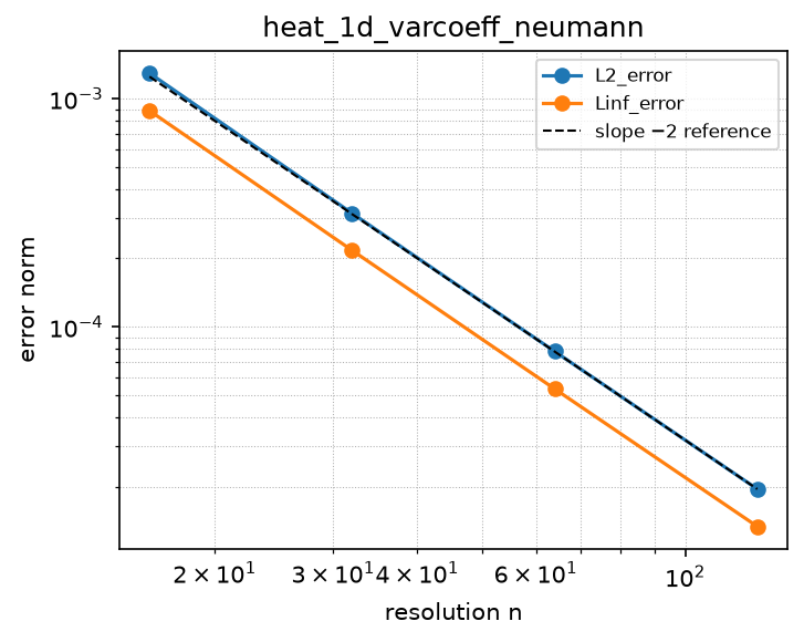
varcoeff_laplacian_periodic
Source: grids/cartesian_uniform_1d/rules/varcoeff_laplacian_periodic.esm
Rewrites ∂(k·∂u/∂x)/∂x at priority 10 — match pattern:
{"op": "D", "args": [{"op": "*", "args": ["k", {"op": "D", "args": ["u"], "wrt": "x"}]}], "wrt": "x"}
where): fires only when u is a bare field shaped [x]; k is a bare field shaped [x]. Under import-edge renaming (§9.7.7) the wrt literal and this shape follow the renamed axis together, so the rule can be imported more than once (each instance scoped to its own grid) without a first-declared-wins collision. A consumer differentiating a compound inline expression must bind it to a declared shaped observed first.Discretization — one makearray tiling the output axes; boundary conditions live in the face regions of this same rule (esm-spec §9.6.8; later regions overwrite earlier, §4.3.2):
| Region | Treatment | Value |
|---|---|---|
x ∈ [2, N−1] | interior | varcoeff_laplacian_interior(u, k)[i] = ((0.5·(k[i] + k[i+1]))·(u[i+1] − u[i]) − (0.5·(k[i−1] + k[i]))·(u[i] − u[i−1])) / dx² for i ∈ [2, N−1] |
x = 1 | boundary face | ((0.5·(k[1] + k[2]))·(u[2] − u[1]) − (0.5·(k[N] + k[1]))·(u[1] − u[N])) / dx² |
x = N | boundary face | ((0.5·(k[N] + k[1]))·(u[1] − u[N]) − (0.5·(k[N−1] + k[N]))·(u[N] − u[N−1])) / dx² |
Conservative finite-volume VARIABLE-COEFFICIENT / NONLINEAR Laplacian div(k grad u) with PERIODIC boundary on cartesian_uniform_1d, cell-centered. Like varcoeff_laplacian_zero_flux_bc the operator carries a coefficient, so a bare laplacian match cannot express it; the rule matches the CONSERVATIVE COMPOUND the consumer writes, D( {op:*, args:[k, D(u,wrt:x)]}, wrt:x ) – outer-D of (k times the inner spatial gradient) – at priority 10, so under esm-spec 9.6.3 outermost-first compound precedence it fires on the whole compound before any plain-D rule could lower the inner derivative (exactly as central_D2_periodic fires on D(D(f,x),x)). BOTH operands are match wildcards bound to consumer fields: u (the state, inner D’s argument) and k (the coefficient, the LEFT factor of the product); matching is structural and non-commutative, so the consumer MUST write the coefficient on the LEFT: k * D(u, wrt:x). Match-scoped with where {u:{shape:[x]}, k:{shape:[x]}} (esm-spec 9.6.1) so it fires only on this grid’s declared x-shaped fields; under import-edge renaming (esm-spec 9.7.7) the wrt literals and both where shapes follow the renamed axis together, so two cartesian instances coexist scoped to their own grids. ONE rule serves two duals: the VARIABLE-COEFFICIENT case (k=k(x), a given periodic field) and the NONLINEAR case (k declared as an observed k=f(u)); the body only reads k by name at the faces, so a state-dependent k just makes the expanded stencil nonlinear in u with no reformulation (the keyed-factor field contract). AUTHORING CONTRACT for k (identical to varcoeff_laplacian_zero_flux_bc): k is a declared x-shaped field; when supplied as an aggregate observed it MUST loop over an index DISTINCT from the stencil’s interior index i (the library convention is gi), because the coefficient observed is inlined into the stencil’s [2,N-1] aggregate at evaluation and a shared loop-index name is captured (silently wrong interior values). Face conductivity is the ARITHMETIC MEAN kf[i+1/2]=(k[i]+k[i+1])/2 (O(dx^2) at the face for a differentiable coefficient, affine in k so it composes with the nonlinear dual). Interior [2, N-1]: the imported conservative flux-difference stencil. The two faces i=1 and i=N carry the same conservative flux difference with the out-of-range neighbor AND its coefficient wrapped periodically: at i=1 the left domain-face flux uses the ghost u[0]=u[N] and k[0]=k[N], giving kf[1/2]=(k[N]+k[1])/2 and L u[1] = ( (k[1]+k[2])/2 (u[2]-u[1]) - (k[N]+k[1])/2 (u[1]-u[N]) ) / dx^2; at i=N the right domain-face flux uses u[N+1]=u[1] and k[N+1]=k[1], giving kf[N+1/2]=(k[N]+k[1])/2 and L u[N] = ( (k[N]+k[1])/2 (u[1]-u[N]) - (k[N-1]+k[N])/2 (u[N]-u[N-1]) ) / dx^2. The SAME wrapped face flux (k[N]+k[1])/2 (u[1]-u[N])/dx is the left face of cell 1 and the right face of cell N, so the discrete operator is exactly conservative (the circulant variable-coefficient Laplacian) and its row sums vanish, preserving the discrete mean – the natural variable-coefficient analogue of central_D2_periodic. dx is a free name resolving to the consuming model’s spacing variable (grids/cartesian_uniform_1d/grid.esm); the periodic wrap is dx-scale-invariant, so the rule serves any domain extent unchanged. Reduces to central_D2_periodic when k is spatially constant. Interior and periodic faces are all O(dx^2), so the whole operator is 2nd order with no boundary reduction. A model imports exactly one second-derivative/Laplacian rule for x.
References
- LeVeque, R. J. (2007). Finite Difference Methods for Ordinary and Partial Differential Equations. SIAM. Section 2.15 (variable-coefficient conservative form) and Section 3 (periodic boundary conditions).
Conformance fixtures
- ast:
varcoeff_laplacian_periodic— statusactive - convergence:
heat_1d_varcoeff_periodic— statusactive - simulation:
heat_1d_varcoeff_periodic— statusactive
Convergence — case heat_1d_varcoeff_periodic
Error norms read from the committed golden tests/conformance/convergence/heat_1d_varcoeff_periodic/golden/errors.json (binding: julia; nothing recomputed for display).
| n | L2_error | observed order | Linf_error | observed order |
|---|---|---|---|---|
| 16 | 4.046e-02 | — | 8.114e-04 | — |
| 32 | 9.975e-03 | 2.02 | 2.028e-04 | 2.00 |
| 64 | 2.485e-03 | 2.01 | 5.069e-05 | 2.00 |
| 128 | 6.207e-04 | 2.00 | 1.267e-05 | 2.00 |
Expected order: 2 (± 0.2).
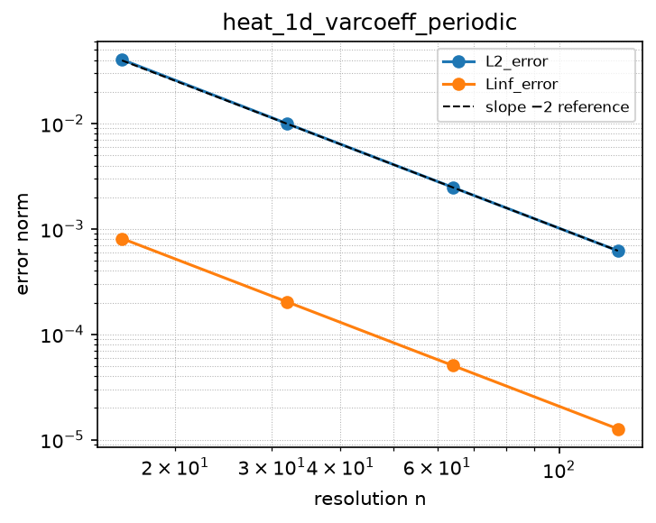
varcoeff_laplacian_zero_flux_bc
Source: grids/cartesian_uniform_1d/rules/varcoeff_laplacian_zero_flux_bc.esm
Rewrites ∂(k·∂u/∂x)/∂x at priority 10 — match pattern:
{"op": "D", "args": [{"op": "*", "args": ["k", {"op": "D", "args": ["u"], "wrt": "x"}]}], "wrt": "x"}
where): fires only when u is a bare field shaped [x]; k is a bare field shaped [x]. Under import-edge renaming (§9.7.7) the wrt literal and this shape follow the renamed axis together, so the rule can be imported more than once (each instance scoped to its own grid) without a first-declared-wins collision. A consumer differentiating a compound inline expression must bind it to a declared shaped observed first.Discretization — one makearray tiling the output axes; boundary conditions live in the face regions of this same rule (esm-spec §9.6.8; later regions overwrite earlier, §4.3.2):
| Region | Treatment | Value |
|---|---|---|
x ∈ [2, N−1] | interior | varcoeff_laplacian_interior(u, k)[i] = ((0.5·(k[i] + k[i+1]))·(u[i+1] − u[i]) − (0.5·(k[i−1] + k[i]))·(u[i] − u[i−1])) / dx² for i ∈ [2, N−1] |
x = 1 | boundary face | ((0.5·(k[1] + k[2]))·(u[2] − u[1])) / dx² |
x = N | boundary face | ((0.5·(k[N−1] + k[N]))·(u[N−1] − u[N])) / dx² |
Conservative finite-volume VARIABLE-COEFFICIENT / NONLINEAR Laplacian div(k grad u) with zero-flux (homogeneous Neumann) boundaries on cartesian_uniform_1d. The operator carries a coefficient, so a bare laplacian match cannot express it; instead the rule matches the CONSERVATIVE COMPOUND the consumer writes, D( {op:, args:[k, D(u,wrt:x)]}, wrt:x ) – outer-D of (k times the inner spatial gradient) – at priority 10, so under esm-spec 9.6.3 outermost-first compound precedence it fires on the whole compound before any plain-D rule could lower the inner derivative (exactly as central_D2_zero_grad_bc fires on D(D(f,x),x)); this mirrors the archive nonlinear_laplacian applies_to grad(fgrad(u)) ported to the esm-spec 0.8.0 D/wrt spelling. BOTH operands are match wildcards bound to consumer fields: u (the state, inner D’s argument) and k (the coefficient, the LEFT factor of the product). Because matching is structural and non-commutative, the consumer MUST write the coefficient on the LEFT: k * D(u, wrt:x); a product spelled D(u,x)*k or a compound coefficient does not match (bind a compound coefficient to a declared x-shaped observed first). Match-scoped with where {u:{shape:[x]}, k:{shape:[x]}} (esm-spec 9.6.1) so it fires only on this grid’s declared x-shaped fields, and under import-edge renaming (esm-spec 9.7.7) the wrt literals and both where shapes follow the renamed axis together, so two cartesian instances coexist scoped to their own grids. ONE rule serves two duals: the VARIABLE-COEFFICIENT case (k=k(x), a given field) and the NONLINEAR case (the consumer declares k as an observed k=f(u), so k depends on the state) – the body only reads k by bare name at the faces, so a state-dependent k just makes the expanded stencil nonlinear in u with no reformulation (the keyed-factor field contract, like the grid’s dx and the nonuniform grid’s xc). AUTHORING CONTRACT for k: it is a declared x-shaped field; when supplied as an aggregate observed (k = aggregate over some index of an expression), that aggregate MUST loop over an index DISTINCT from the stencil’s interior index i, because the coefficient observed is inlined into the stencil’s [2,N-1] aggregate at evaluation and a shared loop-index name is captured (silently wrong interior values). This is the same reason the library’s geometry observeds loop over gi rather than i (grids/cartesian_nonuniform_1d nonuniform_cell_center/width); a consumer coefficient should follow suit (e.g. loop over gi). A k supplied as a plain state/parameter array, a loader field, or a state-dependent observed with a non-i loop index needs no special care. Face conductivity is the ARITHMETIC MEAN kf[i+1/2]=(k[i]+k[i+1])/2 (O(dx^2) at the face for a differentiable coefficient, and affine in k so it composes with the nonlinear dual). Interior [2, N-1]: the imported conservative flux-difference stencil. The boundary faces impose zero flux exactly (natural for the finite-volume form – no ghost geometry): at i=1 the left domain-face flux is dropped, giving L u[1] = kf[3/2](u[2]-u[1])/dx^2 = (k[1]+k[2])/2 (u[2]-u[1])/dx^2; at i=N the right domain-face flux is dropped, giving L u[N] = -kf[N-1/2](u[N]-u[N-1])/dx^2 = (k[N-1]+k[N])/2 (u[N-1]-u[N])/dx^2. dx is a free name resolving to the consuming model’s spacing variable (grids/cartesian_uniform_1d/grid.esm); the zero-flux closure is dx-scale-invariant, so the rule serves any domain extent unchanged. Reduces to central_D2_zero_grad_bc when k is spatially constant. Interior O(dx^2); the one-sided zero-flux faces are O(dx) locally, which preserves global 2nd-order L2 convergence for zero-flux-compatible solutions (flux k u_x vanishing at both walls). A model imports exactly one second-derivative/Laplacian rule for x.
References
- LeVeque, R. J. (2007). Finite Difference Methods for Ordinary and Partial Differential Equations. SIAM. Section 2.15 (variable-coefficient conservative form) and Section 2.12 (Neumann boundary conditions by dropping the domain-face flux).
Conformance fixtures
- ast:
varcoeff_laplacian_zero_flux_bc— statusactive - convergence:
heat_1d_varcoeff_zero_flux— statusactive - simulation:
heat_1d_varcoeff_zero_flux— statusactive
Convergence — case heat_1d_varcoeff_zero_flux
Error norms read from the committed golden tests/conformance/convergence/heat_1d_varcoeff_zero_flux/golden/errors.json (binding: julia; nothing recomputed for display).
| n | L2_error | observed order | Linf_error | observed order |
|---|---|---|---|---|
| 16 | 6.726e-03 | — | 2.584e-03 | — |
| 32 | 1.692e-03 | 1.99 | 6.522e-04 | 1.99 |
| 64 | 4.236e-04 | 2.00 | 1.630e-04 | 2.00 |
| 128 | 1.060e-04 | 2.00 | 4.078e-05 | 2.00 |
Expected order: 2 (± 0.2).
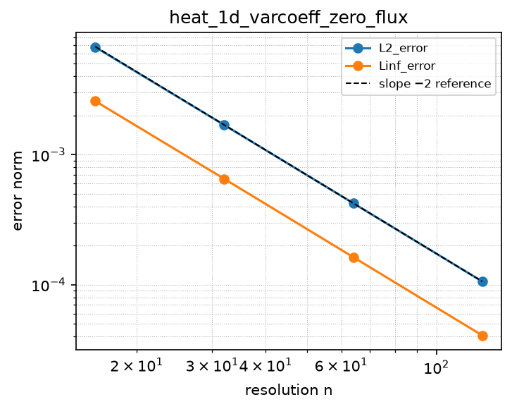
weno5_D_inflow_bc
Source: grids/cartesian_uniform_1d/rules/weno5_D_inflow_bc.esm
Rewrites ∂u/∂x at priority 10 — match pattern:
{"op": "D", "args": ["u"], "wrt": "x"}
where): fires only when u is a bare field shaped [x]. Under import-edge renaming (§9.7.7) the wrt literal and this shape follow the renamed axis together, so the rule can be imported more than once (each instance scoped to its own grid) without a first-declared-wins collision. A consumer differentiating a compound inline expression must bind it to a declared shaped observed first.Discretization — one makearray tiling the output axes; boundary conditions live in the face regions of this same rule (esm-spec §9.6.8; later regions overwrite earlier, §4.3.2):
| Region | Treatment | Value |
|---|---|---|
x ∈ [4, N−2] | interior | weno5_D_interior(u)[i] = (weno5_recon(u[i−2], u[i−1], u[i], u[i+1], u[i+2]) − weno5_recon(u[i−3], u[i−2], u[i−1], u[i], u[i+1])) / dx for i ∈ [4, N−2] |
x = 1 | boundary face | (weno3_recon(gL, u[1], u[2]) − gL) / dx |
x = 2 | boundary face | (weno3_recon(u[1], u[2], u[3]) − weno3_recon(gL, u[1], u[2])) / dx |
x = 3 | boundary face | (weno5_recon(u[1], u[2], u[3], u[4], u[5]) − weno3_recon(u[1], u[2], u[3])) / dx |
x = N−1 | boundary face | (weno3_recon(u[N−2], u[N−1], u[N]) − weno5_recon(u[N−4], u[N−3], u[N−2], u[N−1], u[N])) / dx |
x = N | boundary face | (weno3_recon(u[N−1], u[N], u[N]) − weno3_recon(u[N−2], u[N−1], u[N])) / dx |
Fifth-order upwind (positive transport speed) WENO5-Z first derivative u_x on cartesian_uniform_1d with OPEN boundaries – a prescribed inflow (Dirichlet) value at the upstream (left) wall and a non-reflecting extrapolation outflow at the downstream (right) wall – for advection with non-negative transport speed (a consumer writes u_t = -c*D(u, wrt: x), c >= 0). This is the open-boundary sibling of rules/weno5_D_periodic.esm and, exactly like it and like rules/ppm_D_inflow_bc.esm, is built THINLY on the already-well-factored WENO5 stencil chain (stencils/weno5_D_interior.esm <- stencils/weno5_recon.esm) rather than re-deriving any reconstruction algebra: the interior region [4, N-2] is a SINGLE apply of stencils/weno5_D_interior.esm (the CONSERVATIVE FINITE-DIFFERENCE flux-difference aggregate D u[i] = (hatF_{i+1/2} - hatF_{i-1/2})/dx, Shu 1998, over the six-cell support u[i-3..i+2] with the Jiang-Shu/WENO-Z 5-cell reconstruction hatF = weno5_recon). CONSERVATIVE FLUX-DIFFERENCE FORM IS KEPT IN THE INTERIOR; only the five near-wall cells i in {1,2,3} (inflow) and {N-1, N} (outflow) are explicit makearray faces, and each still holds a conservative flux difference (hatF_{i+1/2} - hatF_{i-1/2})/dx with the face fluxes reconstructed at whatever order the AVAILABLE cells support. REDUCED-ORDER BOUNDARY RECONSTRUCTION (the crux): the 5-cell WENO5 window runs out of interior cells within two cells of each wall, so those faces degrade to the third-order stencils/weno3_recon.esm (WENO3-Z, left-biased 3-cell window, same WENO-Z algebra as weno5_recon so the two are consistent), while every face whose full 5-cell window still fits inside the domain REUSES stencils/weno5_recon.esm unchanged – no new fifth-order algebra is introduced. LEFT INFLOW WALL (i=1,2,3): the wall face flux is hatF_{1/2} = gL – the incoming flux is the prescribed upstream inflow value, NOT a reconstruction contaminated by downstream cells (matching rules/upwind1_D_inflow_bc’s (u[1]-gL)/dx face and rules/ppm_D_inflow_bc’s F_{1/2}=gL). The two near-wall interior faces are WENO3: hatF_{3/2} = weno3_recon(gL, u[1], u[2]) (one upstream ghost = gL) and hatF_{5/2} = weno3_recon(u[1], u[2], u[3]) (fully interior); the first fully-fitting face hatF_{7/2} = weno5_recon(u[1..5]) is already the full fifth-order stencil and is byte-identical to the interior aggregate’s hatF_{i-1/2} at i=4 (shared face -> conservative). RIGHT OUTFLOW WALL (i=N-1, N): NON-REFLECTING – hatF_{(N-2)+1/2} = weno5_recon(u[N-4..N]) is fully interior and byte-identical to the interior aggregate’s hatF_{i+1/2} at i=N-2 (shared face); hatF_{(N-1)+1/2} = weno3_recon(u[N-2], u[N-1], u[N]) is a fully-interior one-sided WENO3; and the outflow wall face hatF_{N+1/2} = weno3_recon(u[N-1], u[N], u[N]) fills the single downstream ghost u[N+1] by zeroth-order extrapolation u[N+1]=u[N], so every right-wall reconstruction reaches only interior/self data – no external condition is imposed where characteristics leave the domain, so no spurious reflection enters and pure advection stays well-posed with the single upstream wall value. CONSERVATION: every interior interface (faces 3/2 through (N-1)/2) is written with byte-identical reconstruction bindings in the two cells that share it, so the flux difference telescopes and mass is conserved to the bit in the interior; the domain is OPEN (mass enters through hatF_{1/2}=gL and leaves through hatF_{N+1/2}), so unlike the periodic ring sum(u) is not globally invariant and there is no mean-conservation claim. The six regions tile [1, N] exactly (needs N >= 6, as in weno5_D_periodic). ORDER (honest, pinned by the sweep, NOT the nominal 5): the interior runs near fifth order on smooth data, but the global observed order is LIMITED BY THE REDUCED-ORDER (WENO3, third-order) boundary reconstruction plus the wall-flux closures – so it is well below 5 and norm-dependent, pinned in tests/conformance/convergence/advection_1d_inflow_weno5 (this is a boundary-reduced order, NOT a fifth-order claim). Free names: gL is the consumer-supplied inflow value at the left wall x = x0 with default 0 (the same contract as rules/upwind1_D_inflow_bc’s gL, rules/ppm_D_inflow_bc’s gL, and the grid geometry dx; an unset parameter falls back to its default per esm-spec 6, so gL = 0 is the zero-inflow case), appearing only in the runtime rule body, never in a build-time ic/reference position (AGENTS.md build-time scope caveat); dx is the grid’s consumer-supplied spacing (grids/cartesian_uniform_1d/grid.esm), and every boundary face is dx-scale-invariant so the rule serves any domain extent unchanged. MATCH: plain D(u, wrt: x) at priority 10 (mirroring the ppm_D_inflow_bc and lax_friedrichs_D_inflow_bc siblings) so it wins over any default-priority first-derivative rule sharing the axis; match-scoped where: {u: {shape: [x]}} (esm-spec 9.6.1) so it fires only on the first derivative of a bare field over this grid’s x index set, and under esm-spec 9.7.7 import renaming the wrt literal and the where shape follow the renamed axis together (two cartesian instances coexist). The constraint requires a bare shaped field; a consumer differentiating a compound expression must bind it to a declared x-shaped observed first. A model imports exactly one advection rule for x. Sign convention: upwind for flow in +x (inflow at the left wall); a sign-mirrored right-inflow variant belongs in a separate rule. The expanded AST is large (the WENO5 nonlinear reconstruction is repeated per face); like weno5_D_periodic its AST golden is pinned by sha256 digest above the 64 KiB threshold, and bindings that hang on the huge nonlinear RHS are recorded as blocked_upstream_bindings in the simulation/convergence manifests by analogy to weno5_D_periodic.
References
- Jiang, G.-S., & Shu, C.-W. (1996). Efficient Implementation of Weighted ENO Schemes. Journal of Computational Physics, 126(1), 202-228. The fifth-order interior reconstruction and its third-order reduction used at the walls.
doi:10.1006/jcph.1996.0130 - Shu, C.-W. (1998). Essentially Non-Oscillatory and Weighted Essentially Non-Oscillatory Schemes for Hyperbolic Conservation Laws. Lecture Notes in Mathematics 1697, 325-432. The conservative finite-difference flux-reconstruction framework D u[i] = (hatF_{i+1/2}-hatF_{i-1/2})/dx.
doi:10.1007/BFb0096355 - Borges, R., Carmona, M., Costa, B., & Don, W. S. (2008). An improved weighted essentially non-oscillatory scheme for hyperbolic conservation laws. Journal of Computational Physics, 227(6), 3191-3211. The WENO-Z nonlinear weights used in both the interior (weno5_recon) and boundary (weno3_recon) reconstructions.
doi:10.1016/j.jcp.2007.11.038 - LeVeque, R. J. (2002). Finite Volume Methods for Hyperbolic Problems. Cambridge University Press. Section 7 (inflow / outflow boundary conditions for advection); the prescribed-inflow and non-reflecting-outflow closures used at the two walls.
Conformance fixtures
- ast:
weno5_D_inflow_bc— statusactive - convergence:
advection_1d_inflow_weno5— statusactive - simulation:
advection_1d_inflow_weno5— statusactive
Convergence — case advection_1d_inflow_weno5
Error norms read from the committed golden tests/conformance/convergence/advection_1d_inflow_weno5/golden/errors.json (binding: julia; nothing recomputed for display).
| n | L2_error | observed order | Linf_error | observed order |
|---|---|---|---|---|
| 16 | 4.633e-03 | — | 7.017e-03 | — |
| 32 | 1.015e-03 | 2.19 | 2.057e-03 | 1.77 |
| 64 | 1.573e-04 | 2.69 | 4.833e-04 | 2.09 |
| 128 | 1.242e-05 | 3.66 | 3.936e-05 | 3.62 |
Expected order: 2.4 (± 0.4).
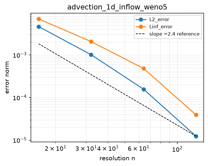
weno5_D_periodic
Source: grids/cartesian_uniform_1d/rules/weno5_D_periodic.esm
Rewrites ∂u/∂x — match pattern:
{"op": "D", "args": ["u"], "wrt": "x"}
where): fires only when u is a bare field shaped [x]. Under import-edge renaming (§9.7.7) the wrt literal and this shape follow the renamed axis together, so the rule can be imported more than once (each instance scoped to its own grid) without a first-declared-wins collision. A consumer differentiating a compound inline expression must bind it to a declared shaped observed first.Discretization — one makearray tiling the output axes; boundary conditions live in the face regions of this same rule (esm-spec §9.6.8; later regions overwrite earlier, §4.3.2):
| Region | Treatment | Value |
|---|---|---|
x ∈ [4, N−2] | interior | weno5_D_interior(u)[i] = (weno5_recon(u[i−2], u[i−1], u[i], u[i+1], u[i+2]) − weno5_recon(u[i−3], u[i−2], u[i−1], u[i], u[i+1])) / dx for i ∈ [4, N−2] |
x = 1 | boundary face | (weno5_recon(u[N−1], u[N], u[1], u[2], u[3]) − weno5_recon(u[N−2], u[N−1], u[N], u[1], u[2])) / dx |
x = 2 | boundary face | (weno5_recon(u[N], u[1], u[2], u[3], u[4]) − weno5_recon(u[N−1], u[N], u[1], u[2], u[3])) / dx |
x = 3 | boundary face | (weno5_recon(u[1], u[2], u[3], u[4], u[5]) − weno5_recon(u[N], u[1], u[2], u[3], u[4])) / dx |
x = N−1 | boundary face | (weno5_recon(u[N−3], u[N−2], u[N−1], u[N], u[1]) − weno5_recon(u[N−4], u[N−3], u[N−2], u[N−1], u[N])) / dx |
x = N | boundary face | (weno5_recon(u[N−2], u[N−1], u[N], u[1], u[2]) − weno5_recon(u[N−3], u[N−2], u[N−1], u[N], u[1])) / dx |
Fifth-order upwind (positive transport speed) WENO5-Z first derivative with a periodic boundary on cartesian_uniform_1d, for advection u_t = -c u_x (c >= 0). Conservative finite-difference form (Shu 1998): D(u,x)|i = (hatF{i+1/2} - hatF_{i-1/2})/dx with the Jiang-Shu (1996) WENO5 flux reconstruction and WENO-Z (Borges 2008) nonlinear weights; see stencils/weno5_D_interior.esm for the full closed-form reconstruction and the order argument. The complete derivative reads u[i-3..i+2] (the WENO reconstruction stencil is 5 cells wide; the flux difference spans 6). The interior aggregate covers i in [4, N-2] where all six cells are in range; the near-boundary cells i in {1,2,3} and {N-1, N} are explicit makearray faces holding the same conservative flux difference with the out-of-range neighbors wrapped PERIODICALLY (index j<1 -> j+N, j>N -> j-N), following the ESS pde_simulation periodic-boundary precedent (upwind1_D_periodic, godunov_norm_D1_periodic). Three wrap cells are needed on the left and two on the right because the conservative stencil is left-biased (u[i-3] is the farthest-reaching point). The six regions tile [1, N] exactly. Matches plain D(u, wrt: x) at default priority, exactly like the first-derivative siblings upwind1_D_periodic and central_D1_periodic (identical match and where): the three are alternative discretizations distinguished by which one the consuming model imports, not by priority; a model imports exactly one first-derivative rule for x, so they never compete within a document. Match-scoped with where: {u: {shape: [x]}} (esm-spec 9.6.1) so it fires only on the first derivative of a bare field declared over this grid’s x index set; under import-edge renaming (esm-spec 9.7.7) the wrt literal and the where shape follow the renamed axis together, so two cartesian instances coexist scoped to their own grids. The constraint requires a bare shaped variable, so a consumer differentiating a compound expression must bind it to a declared x-shaped observed first. dx is a free name resolving to the consuming model’s spacing variable (grids/cartesian_uniform_1d/grid.esm consumer-supplied geometry contract); the periodic wrap is dx-scale-invariant, so the rule serves any domain extent unchanged. O(dx^5) on smooth data (verified: leading smooth-limit truncation error -(dx^5/60) u^(6)); WENO-Z preserves fifth order through the critical points of a smooth periodic profile.
References
- Jiang, G.-S., & Shu, C.-W. (1996). Efficient Implementation of Weighted ENO Schemes. Journal of Computational Physics, 126(1), 202-228. Smoothness indicators beta_k (eq. 2.17), nonlinear weights (eqs. 2.9-2.10), and the fifth-order reconstruction.
doi:10.1006/jcph.1996.0130 - Shu, C.-W. (1998). Essentially Non-Oscillatory and Weighted Essentially Non-Oscillatory Schemes for Hyperbolic Conservation Laws. In Advanced Numerical Approximation of Nonlinear Hyperbolic Equations, Lecture Notes in Mathematics 1697, 325-432. NASA/CR-97-206253. The conservative finite-difference flux-reconstruction framework: f’(x_i) = (hatf_{i+1/2} - hatf_{i-1/2})/dx with hatf reconstructed from the sliding-average primitive, eqs. (2.16)-(2.18).
doi:10.1007/BFb0096355 - Borges, R., Carmona, M., Costa, B., & Don, W. S. (2008). An improved weighted essentially non-oscillatory scheme for hyperbolic conservation laws. Journal of Computational Physics, 227(6), 3191-3211. The WENO-Z weights alpha_k = d_k (1 + (tau_5/(eps+beta_k))^2) with tau_5 = |beta_0 - beta_2|, which recover the full fifth order at first-order critical points where the classic Jiang-Shu weights degrade.
doi:10.1016/j.jcp.2007.11.038 - Henrick, A. K., Aslam, T. D., & Powers, J. M. (2005). Mapped weighted essentially non-oscillatory schemes: Achieving optimal order near critical points. Journal of Computational Physics, 207(2), 542-567. The demonstration that classic WENO5 drops to fourth order at simple critical points (u’=0, u’’!=0), motivating the WENO-Z remedy used here.
doi:10.1016/j.jcp.2005.01.023
Conformance fixtures
- ast:
weno5_D_periodic— statusactive - convergence:
advection_1d_periodic_weno5— statusactive - simulation:
advection_1d_periodic_weno5— statusactive
Convergence — case advection_1d_periodic_weno5
Error norms read from the committed golden tests/conformance/convergence/advection_1d_periodic_weno5/golden/errors.json (binding: julia; nothing recomputed for display).
| n | L2_error | observed order | Linf_error | observed order |
|---|---|---|---|---|
| 16 | 9.855e-05 | — | 9.747e-05 | — |
| 32 | 3.041e-06 | 5.02 | 3.007e-06 | 5.02 |
| 64 | 9.536e-08 | 5.00 | 9.526e-08 | 4.98 |
| 128 | 2.983e-09 | 5.00 | 2.983e-09 | 5.00 |
Expected order: 5 (± 0.3).