latlon3d
Three-dimensional longitude-latitude-level grid: the 2-D grids/latlon horizontal mesh extended with a vertical lev axis, for 3-D tracer transport on a lat-lon model such as GEOS-Chem Classic. The lon, lat, lev index sets are the iteration axes; NLON, NLAT, NLEV (the point/cell counts) are the esm-spec 9.7 metaparameters, bound at an import edge or the loader API. HORIZONTAL geometry is INHERITED from grids/latlon by expression_template_imports (../latlon/grid.esm): the templates lon_coord, lat_coord, coslat, deg2rad and the free-name contract are reused verbatim, so the horizontal conventions are IDENTICAL to grids/latlon — longitude CELL-based with centers lon_i = lon0_deg + (i - 1/2) dlon_deg (i = 1..NLON), closing into a periodic zonal circle when NLON dlon_deg = 360; latitude POINT-based, endpoint-inclusive, lat_j = lat0_deg + (j - 1) dlat_deg (j = 1..NLAT), pole to pole on the global recipe (lat0_deg = -90, dlat_deg = 180/(NLAT-1)). The real-valued horizontal geometry (lon0_deg, dlon_deg, lat0_deg, dlat_deg, R_sphere) stays consumer-supplied free names, exactly as in grids/latlon. The lon/lat/lon_nodes/lat_nodes index sets and the NLON/NLAT metaparameters are ALSO declared locally here (deep-equal with the import) because the tags-contract lint (validate-library L006) reads a grid file’s own literal index_sets/metaparameters and does not resolve imports. VERTICAL geometry follows the grids/cartesian_nonuniform_1d ‘grid owns the edge->center/thickness derivation’ (Design-B) pattern: lev is a CELL axis of NLEV cells and lev_nodes is its N+1 EDGE axis (sized {op:+, args:[NLEV,1]}, an esm-spec 9.7.6 metaparameter-expression folded at load). The vertical geometry is NOT baked in — a consuming model supplies a SINGLE 1-D edge array pe (shape [lev_nodes], the vertical coordinate at level edges, monotone increasing with the lev index) and the grid derives cell centers lev_center = (pe[k]+pe[k+1])/2 and control thicknesses lev_thickness = pe[k+1]-pe[k] through two match-less templates a consumer applies to its pe (the keyed-factor contract grids/mpas uses for areaCell/dvEdge and grids/cartesian_nonuniform_1d uses for xc/dxw). The geometry aggregate index is gk (NOT k) so a derived dp/zc observed does not capture a consuming vertical stencil’s own aggregate index k when it is inlined (the non-hygienic-inlining footgun documented in grids/cartesian_nonuniform_1d). GEOS-CHEM CLASSIC RECIPE: horizontally the standard 4x5 / 2x2.5 / nested resolutions map onto the latlon contract directly — the GEOS-Chem latitude CENTERS (e.g. -90, -86, …, 86, 90 at 4x5) ARE the uniform pole-to-pole points lat_j = -90 + (j-1) dlat_deg, so the per-degree finite-difference operators here read the correct center coordinates; GEOS-Chem’s HALF-POLAR polar caps are a cell-WIDTH (area/flux-weighting) property that affects only the conservative flux-form transport, not the advective-form per-degree derivative; they are no longer deferred but are DERIVED from the point latitudes by the inherited lat_edge clamp — see the HORIZONTAL FACE AXES paragraph below. Vertically GEOS-Chem uses a hybrid sigma-pressure (eta) coordinate with pressure at level edges P_edge = Ap + Bp*Psurf (Ap in hPa, Bp dimensionless; 72 or reduced 47 levels); a consumer supplies pe from that table. V1 SCOPE (this grid): the vertical spacing is a 1-D COLUMN PROFILE dp = dp(k) — supply pe for a representative column (Psurf constant, or a pure-pressure region where Bp = 0), for which pe is a genuine 1-D array; the FULL Psurf-coupled 3-D thickness dp[i,j,k] (true terrain-following hybrid) is a documented follow-on (expressible as a rank-3 keyed factor, deferred with the conservative flux-form work). SCHEME CAVEAT: the rules on this grid are METHOD-OF-LINES spatial operators (each supplies one directional D(q, wrt: axis); the ODE integrator owns dt), composed by the consumer into du/dt = -(u D(q,lon) + v D(q,lat) + w D(q,lev)); this is NOT the fully-discrete flux-form semi-Lagrangian TPCORE scheme GEOS-Chem uses operationally (Lin & Rood 1996), which carries the Courant number inside the operator and cannot be expressed method-of-lines — see grids/cartesian_uniform_1d/rules/ppm_D_periodic for the same semi-discrete-vs-Courant distinction. HORIZONTAL FACE AXES AND THE HALF-POLAR CAPS (inherited from grids/latlon; the index sets are mirrored literally below). Alongside lev_nodes this grid carries the two HORIZONTAL N+1 edge axes lon_nodes (NLON+1) and lat_nodes (NLAT+1). They hold the face-staggered horizontal winds and the face metrics of the conservative flux-form operators; face j is the LOWER (southern) edge of cell j and face i the western edge of cell i — the same convention as face k = lower edge of cell k in the vertical — so faces 1 and NLAT+1 are the two meridional walls. lon_nodes is declared now so the contract is frozen ahead of the zonal flux-form work; no rule here reads it yet. Because latitude is POINT-based it has no native edges, so the grid MANUFACTURES them with the clamped-midpoint rule of the inherited lat_edge template: phie[j] = max(lat0_deg, min(latN_deg, lat0_deg + (j - 1.5) dlat_deg)), latN_deg = lat0_deg + (NLAT - 1) dlat_deg — interior edges are midpoints of neighbouring points, the two end edges CLAMP to the domain ends, and on the global recipe that clamp is exactly what produces GEOS-Chem’s HALF-POLAR CAPS (the j = 1 and j = NLAT rows span half a nominal interval). The derived geometry follows the SAME keyed-factor contract as pe -> lev_thickness/lev_center: the CONSUMER declares one observed phie (shape [lat_nodes], degrees) by applying lat_edge, then feeds that same phie to coslat_edge (shape [lat_nodes]; face-length weight cos(rad(phie))), latcell_area (shape [lat]; the EXACT spherical area weight sin(rad(phie[j+1])) - sin(rad(phie[j]))) and latcell_dphi (shape [lat]; cell width in radians, a HALF-width at the caps). lat0_deg and dlat_deg stay consumer-supplied free names. AGGREGATE-INDEX HYGIENE: those four templates use FOUR DIFFERENT aggregate indices (gje / gjc / gja / gjd) — never j, for the same non-hygienic-inlining reason as gk in the vertical, and never each other’s, because a consumer that shares the producer’s index name has its OFFSET gather phie[gj+1] captured and silently reduced to phie[gj], which makes latcell_area return exact zeros (a silent divide-by-zero, not an error). THE POLE FACES ARE NEVER READ: cos(-/+pi/2) is 6.1e-17 in IEEE double, not 0, so the flux-form lat rules OMIT the two pole-wall flux terms entirely instead of multiplying them by a near-zero face length — the polar no-flux wall is then exact in floating point, and whatever a consumer stores in the pole faces of a [lon, lat_nodes, lev] meridional wind is simply ignored.
BUILD-TIME SCOPE CAVEAT (AGENTS.md): lon_coord/lat_coord/lev_center resolve in RUNTIME positions (rule bodies, equation RHS) but NOT in ic equations or esm-spec 6.6.5 test references, which are evaluated build-time and cellwise with the consumer’s parameters/observeds out of scope — there, coordinates must fold from literals plus the metaparameter names.
Metaparameters
| Name | Type | Default | Description |
|---|---|---|---|
NLON | integer | 144 | Number of cells along longitude (cell-based axis; the global recipe closes the zonal circle with dlon_deg = 360/NLON). |
NLAT | integer | 91 | Number of points along latitude (point-based, endpoint-inclusive axis; the global recipe is pole-to-pole with dlat_deg = 180/(NLAT - 1)). |
NLEV | integer | 72 | Number of vertical cells (levels). Default 72 = the GEOS-Chem native level count (reduced grid: 47). The edge axis lev_nodes has NLEV+1 members. |
All sizes are load-time metaparameters (esm-spec §9.7.6): rebind them at the import edge (or through the loader API) and the same files serve every resolution.
Consumer-supplied free names
Region-generic: the same files serve a global or a regional grid depending on the free-name values the consumer supplies. GLOBAL recipe — lon0_deg = 0, dlon_deg = 360/NLON, lat0_deg = −90, dlat_deg = 180/(NLAT − 1) (pole-to-pole; the zonal circle closes, so the periodic-lon rule applies). REGIONAL recipe — any other origin/spacing (e.g. lon0_deg = −130, dlon_deg = 0.25 over CONUS); the circle does not close, so use the zero-gradient lon rule. Spell the spacings as observeds dividing by the metaparameter names (NLON/NLAT) so a convergence sweep stays consistent. A further free name R_sphere (sphere radius, m) enters only the consumer’s physical-units metric composition (per-degree derivatives → per-metre; the coslat template supplies cos(lat)).
Index sets
| Name | Kind | Size |
|---|---|---|
lon | interval | NLON |
lat | interval | NLAT |
lev | interval | NLEV |
lon_nodes | interval | {'op': '+', 'args': ['NLON', 1]} |
lat_nodes | interval | {'op': '+', 'args': ['NLAT', 1]} |
lev_nodes | interval | {'op': '+', 'args': ['NLEV', 1]} |
Geometry templates
| Template | Definition | Description |
|---|---|---|
lev_center | lev_center[gk] = 0.5·(pe[gk] + pe[gk+1]) for gk ∈ lev | Cell (level) centers from the edge array: lev_center[gk] = (pe[gk] + pe[gk+1]) / 2 over the lev (cell) axis, gathering the NLEV+1-node edge array pe (shape [lev_nodes]). A consuming model applies this to its pe to define its lev-shaped zc observed. The aggregation index is gk, NOT k, so the derived observed does not capture a consuming vertical stencil’s own aggregate index k when inlined (the non-hygienic-inlining footgun; see grids/cartesian_nonuniform_1d/nonuniform_cell_center). |
lev_thickness | lev_thickness[gk] = pe[gk+1] − pe[gk] for gk ∈ lev | Finite-volume control thicknesses from the edge array: lev_thickness[gk] = pe[gk+1] - pe[gk] over the lev (cell) axis. A consuming model applies this to its pe to define its lev-shaped dp observed (positive when pe is monotone increasing with the lev index — the required orientation). Aggregation index gk (distinct from a rule’s k) for the same hygiene reason as lev_center. |
lev_thickness_3d | lev_thickness_3d[gi,gj,gk] = pe[gi, gj, gk+1] − pe[gi, gj, gk] for gi ∈ lon, gj ∈ lat, gk ∈ lev | TERRAIN-FOLLOWING (rank-3) control thicknesses from a THREE-DIMENSIONAL edge array: lev_thickness_3d[gi,gj,gk] = pe[gi,gj,gk+1] - pe[gi,gj,gk] over [lon, lat, lev], gathering the [lon, lat, lev_nodes] edge array pe. This is the Psurf-coupled hybrid-sigma-pressure counterpart of lev_thickness: a consuming model builds a 3-D pressure-at-edges pe[i,j,kn] = Ap[kn] + Bp[kn]*Ps(i,j,t) (which varies in longitude, latitude and time whenever the surface pressure does) and applies this template to define its [lon,lat,lev]-shaped dp observed (positive when pe increases with the lev index — the required orientation). The physical dp is the reconstruction width consumed by the terrain-following flux-form vertical operators (ppm_flux_D_lev_mono_hybrid_noflux_bc). Aggregation indices gi/gj/gk (distinct from a rule’s i/j/k) for the non-hygienic-inlining reason documented on lev_center and lev_thickness. |
Stencils
Interior-only, match-less templates importing grid.esm; the rules below wrap them with boundary-condition face regions into complete rewrite rules.
central_D_lat_interior
Source: grids/latlon3d/stencils/central_D_lat_interior.esm
Interior-only centered first derivative along latitude on the latlon3d grid: (f[i,j+1,k] - f[i,j-1,k]) / (2 dlat_deg) over all i (lon), j in [2, NLAT-1], all k (lev) — a PER-DEGREE derivative (see grids/latlon3d/grid.esm for the physical-units metric recipe). The rank-3 extension of grids/latlon/stencils/central_D_lat_interior, evaluated on every lev level. Match-less named template consumed by the boundary-condition layer (rules/central_D_lat_zero_grad_bc adds the j=1 and j=NLAT pole rows via factored face stencils). dlat_deg is a free name resolving to the consuming model’s meridional spacing variable (the inherited grids/latlon consumer-supplied geometry contract). O(dlat_deg^2) on this uniform axis.
References
- Fornberg, B. (1988). Generation of finite difference formulas on arbitrarily spaced grids. Mathematics of Computation 51(184), 699-706.
doi:10.1090/S0025-5718-1988-0935077-0
central_D_lat_pole_face_hi
Source: grids/latlon3d/stencils/central_D_lat_pole_face_hi.esm
Zero-gradient pole-row closure for the HIGH latitude boundary (j=NLAT, the north pole on the global recipe) of the centered latitude derivative on the latlon3d grid: the one-sided difference (f[i,NLAT,k] - f[i,NLAT-1,k]) / dlat_deg over all i (lon), all k (lev). Match-less named face template consumed by rules/central_D_lat_zero_grad_bc, the high-latitude companion to central_D_lat_pole_face_lo. Produces a full (NLON x 1 x NLEV) slab AGGREGATE at row NLAT. Encodes the zero-gradient (crude pole) condition; superconvergent on a boundary-compatible solution (see problems/latlon3d_advection_meridional_zero_grad). dlat_deg is the inherited consumer-supplied meridional spacing free name.
References
- LeVeque, R. J. (2007). Finite Difference Methods for Ordinary and Partial Differential Equations. SIAM. Section 2.12 (one-sided boundary treatment).
central_D_lat_pole_face_lo
Source: grids/latlon3d/stencils/central_D_lat_pole_face_lo.esm
Zero-gradient pole-row closure for the LOW latitude boundary (j=1, the south pole on the global recipe) of the centered latitude derivative on the latlon3d grid: the one-sided difference (f[i,2,k] - f[i,1,k]) / dlat_deg over all i (lon), all k (lev). Match-less named face template consumed by rules/central_D_lat_zero_grad_bc, which tiles [lon,lat,lev] with the centered interior stencil (rows [2,NLAT-1]) plus this low face (row 1) and the high face (row NLAT). Factored into its own stencil (rather than inlined in the rule) as the compositional face-factoring idiom, here producing a full (NLON x 1 x NLEV) slab AGGREGATE (a lat face is a 2-D slab on a 3-D grid). Encodes the zero-gradient (crude pole) condition; on a boundary-compatible solution whose first Phi-derivatives vanish at the pole the one-sided face is superconvergent and the global scheme stays O(dlat_deg^2) (see problems/latlon3d_advection_meridional_zero_grad). dlat_deg is the inherited consumer-supplied meridional spacing free name.
References
- LeVeque, R. J. (2007). Finite Difference Methods for Ordinary and Partial Differential Equations. SIAM. Section 2.12 (one-sided boundary treatment).
central_D_lev_bottom_face
Source: grids/latlon3d/stencils/central_D_lev_bottom_face.esm
Zero-gradient BOTTOM (k=1, the surface on a hybrid vertical) closure for the vertical centered derivative on the latlon3d grid: the exact second-order ONE-SIDED (forward) nonuniform first derivative (Fornberg 1988) on the three lowest level centers zc[1], zc[2], zc[3], applied to f[i,j,1], f[i,j,2], f[i,j,3] over all i (lon), all j (lat) – a full (NLON x NLAT x 1) slab AGGREGATE. Match-less face template consumed by rules/central_D_lev_zero_grad_bc, the compositional low-boundary companion to central_D_lev_top_face; second order at the wall with no ghost level, the natural no-flux/zero-gradient-compatible closure for a profile whose vertical gradient vanishes at the boundary (see problems/latlon3d_advection_vertical_zero_grad). zc is the consumer free-name center array; only literal-indexed centers are read here, so no aggregate-index capture arises.
References
- Fornberg, B. (1988). Generation of finite difference formulas on arbitrarily spaced grids. Mathematics of Computation 51(184), 699-706.
doi:10.1090/S0025-5718-1988-0935077-0 - LeVeque, R. J. (2007). Finite Difference Methods for Ordinary and Partial Differential Equations. SIAM. Sections 2.13 (nonuniform grids) and 2.12 (one-sided boundary closures).
central_D_lev_interior
Source: grids/latlon3d/stencils/central_D_lev_interior.esm
Interior-only 3-point centered first derivative along the vertical (lev) axis on the latlon3d grid, evaluated on every (lon, lat) column: D f[i,j,k] = -b/(a(a+b)) f[i,j,k-1] + (b-a)/(ab) f[i,j,k] + a/(b(a+b)) f[i,j,k+1] over k in [2, NLEV-1], with a = zc[k]-zc[k-1] and b = zc[k+1]-zc[k] the two center-to-center vertical spacings – the exact Fornberg (1988) 1st-derivative weights on the three unequally spaced level centers zc[k-1], zc[k], zc[k+1]. The rank-3 vertical analogue of grids/cartesian_nonuniform_1d/stencils/central_D1_nonuniform_interior. zc (level centers, shape [lev]) is a free-name array resolving to the consuming model’s geometry observed (defined by applying the grid’s lev_center template to the level-edge array pe; grids/latlon3d/grid.esm) – a first derivative needs only centers, not the thicknesses dp. Match-less; the boundary layer (rules/central_D_lev_zero_grad_bc) adds the k=1 and k=NLEV faces. Second-order in L2 on a smoothly stretched vertical mesh (supraconvergence); reduces to (f[k+1]-f[k-1])/(2 dz) when the levels are uniform. NOTE the zc geometry observed uses the hygienic aggregate index gk (grids/latlon3d lev_center), distinct from this stencil’s k, so its inlining does not capture k.
References
- Fornberg, B. (1988). Generation of finite difference formulas on arbitrarily spaced grids. Mathematics of Computation 51(184), 699-706.
doi:10.1090/S0025-5718-1988-0935077-0 - LeVeque, R. J. (2007). Finite Difference Methods for Ordinary and Partial Differential Equations. SIAM. Sections 2.13 (nonuniform grids) and 2.12 (one-sided boundary closures).
central_D_lev_top_face
Source: grids/latlon3d/stencils/central_D_lev_top_face.esm
Zero-gradient TOP (k=NLEV, the model top/rigid lid on a hybrid vertical) closure for the vertical centered derivative on the latlon3d grid: the exact second-order ONE-SIDED (backward) nonuniform first derivative (Fornberg 1988) on the three highest level centers zc[NLEV-2], zc[NLEV-1], zc[NLEV], applied to f[i,j,NLEV-2], f[i,j,NLEV-1], f[i,j,NLEV] over all i (lon), all j (lat) – a full (NLON x NLAT x 1) slab AGGREGATE. Match-less face template consumed by rules/central_D_lev_zero_grad_bc, the high-boundary companion to central_D_lev_bottom_face. Second order at the wall; no-flux/zero-gradient-compatible. zc is the consumer free-name center array.
References
- Fornberg, B. (1988). Generation of finite difference formulas on arbitrarily spaced grids. Mathematics of Computation 51(184), 699-706.
doi:10.1090/S0025-5718-1988-0935077-0 - LeVeque, R. J. (2007). Finite Difference Methods for Ordinary and Partial Differential Equations. SIAM. Sections 2.13 (nonuniform grids) and 2.12 (one-sided boundary closures).
central_D_lon_interior
Source: grids/latlon3d/stencils/central_D_lon_interior.esm
Interior-only centered first derivative along longitude on the latlon3d grid: (f[i+1,j,k] - f[i-1,j,k]) / (2 dlon_deg) over i in [2, NLON-1], all j (lat), all k (lev) — a PER-DEGREE derivative (see grids/latlon3d/grid.esm for the physical-units metric recipe). The rank-3 extension of grids/latlon/stencils/central_D_lon_interior, evaluated on every lev level, and the zonal sibling of ./central_D_lat_interior. Match-less named template consumed by the boundary-condition layer (rules/central_D_lon_periodic adds the i=1 and i=NLON wrap columns). dlon_deg is a free name resolving to the consuming model’s zonal spacing variable (the inherited grids/latlon consumer-supplied geometry contract). O(dlon_deg^2) on this uniform axis.
References
- Fornberg, B. (1988). Generation of finite difference formulas on arbitrarily spaced grids. Mathematics of Computation 51(184), 699-706.
doi:10.1090/S0025-5718-1988-0935077-0
facediv_lat_cap_n
Source: grids/latlon3d/stencils/facediv_lat_cap_n.esm
NORTH POLAR CAP row (j = NLAT) of the meridional divergence of a face-staggered flux, closed with a ZERO-LENGTH POLE FACE (no flux through the pole): D[i,NLAT,k] = -My[i,NLAT,k] coslat_e[NLAT] / dS_lat[NLAT]. As at the south cap the pole-wall term My[i,NLAT+1,k] coslat_e[NLAT+1] is LITERALLY ABSENT rather than formed and multiplied by cos(+pi/2) = 6.1e-17, and the negation is applied to the single remaining weighted flux – the identical position in which the companion tracer slab upwind1_D_lat_flux_cap_n negates its own single remaining weighted flux. My[i,NLAT+1,k] is never read.
TOGETHER THE TWO CAPS MAKE THE SPHERE A CLOSED SURFACE. Summing dS_lat[j] D[i,j,k] over j = 1..NLAT telescopes to zero exactly: every interior face term My[i,j,k] coslat_e[j] appears once with each sign, written byte-identically in the two rows that share the face, and neither pole term is ever formed. The zonal ring of air mass is therefore conserved to the last bit, and a consumer’s total-mass diagnostic is flat rather than drifting. This is the property that makes the operator usable as the continuity half of a CWC transport pair, and it is the meridional counterpart of the closed-column argument in facediv_lev_nf_kN.
CONSISTENCY WITH CONTINUITY at the north cap follows the same argument as at the south: with q == 1 the donor-cell flux collapses bitwise to the mass flux, the same coslat_e[NLAT] multiplies it, the same dS_lat[NLAT] divides it, and the same unary negation wraps it – so the tracer slab and this slab emit the identical double-precision number and mq tracks m exactly.
GEOMETRY, FACE INDEXING AND FREE NAMES are exactly as in facediv_lat_interior and facediv_lat_cap_s: face j is the southern edge of cell j, so the north cap’s only real face is its SOUTHERN one (face NLAT), My is positive northward, and coslat_e / dS_lat are the consumer’s observeds built from the grid’s coslat_edge and latcell_area templates.
References
- Lin, S.-J., & Rood, R. B. (1996). Multidimensional flux-form semi-Lagrangian transport schemes. Monthly Weather Review, 124(9), 2046-2070.
doi:10.1175/1520-0493(1996)124<2046:MFFSLT>2.0.CO;2 - Jockel, P., von Kuhlmann, R., Lawrence, M. G., et al. (2001). On a fundamental problem in implementing flux-form advection schemes for tracer transport in 3-dimensional general circulation and chemistry transport models. Quarterly Journal of the Royal Meteorological Society, 127(573), 1035-1052.
doi:10.1002/qj.49712757318 - Jacobson, M. Z. (2005). Fundamentals of Atmospheric Modeling (2nd ed.). Cambridge University Press. Chapter 6 (finite-volume flux-form tracer transport; consistency with continuity).
facediv_lat_cap_s
Source: grids/latlon3d/stencils/facediv_lat_cap_s.esm
SOUTH POLAR CAP row (j = 1) of the meridional divergence of a face-staggered flux, closed with a ZERO-LENGTH POLE FACE (no flux through the pole): D[i,1,k] = My[i,2,k] coslat_e[2] / dS_lat[1]. The south pole-wall term My[i,1,k] coslat_e[1] is LITERALLY ABSENT from the lowered expression rather than formed and multiplied by the pole face length.
THAT OMISSION IS THE WHOLE POINT, AND IT IS NOT COSMETIC. On the global recipe the pole face length is coslat_edge(-90 deg) = cos(-pi/2), which in IEEE double is 6.1e-17 – NOT zero. An operator that formed the wall term and multiplied it by that factor would (a) leak a tiny nonzero air mass across the pole, spoiling the exact telescoping of the meridional mass budget, and (b) break the BITWISE agreement with the companion tracer slab upwind1_D_lat_flux_cap_s, which omits its own pole flux outright. Omitting the term makes the polar wall EXACT in floating point and makes the no-flux condition GEOMETRY (a zero-length face) rather than a boundary hack. Consequently My[i,1,k] is NEVER READ: whatever a consumer stores in the pole face of the mass flux is ignored, so a nonzero value there is harmless rather than a silent mass leak.
CONSISTENCY WITH CONTINUITY. With a constant tracer q == 1 the donor-cell flux of upwind1_D_lat_flux_cap_s collapses BITWISE to the mass flux (F = 1/2[My(1+1) - |My|(1-1)] = My, every IEEE step exact), and that slab then multiplies it by coslat_e[2] and divides by dS_lat[1] – the identical two operations, in the identical order, that this slab applies. The two therefore emit the identical double-precision number and the tracer mass mq tracks the air mass m to the last bit at the cap.
THE CAP IS A HALF CELL. Its area weight dS_lat[1] = sin(phi_e[2]) - sin(-pi/2) is O(dphi^2/8) while the single face bounding it to the north has length coslat_e[2] = O(dphi/2). For the CONTINUITY operator that ratio is not an accuracy problem at all – this stencil has no truncation error on cell means, since the exact integral of the flux divergence over the cap IS the single face flux divided by the cap area – but it is exactly the O(1/dphi) amplification that makes the companion ADVECTION operator’s polar accuracy delicate (see the ACCURACY AT THE POLES section of grids/latlon3d/rules/upwind1_flux_D_lat_polar).
GEOMETRY, FACE INDEXING AND FREE NAMES are exactly as in facediv_lat_interior: face j is the southern edge of cell j, faces 1 and NLAT+1 are the poles, My is positive northward, coslat_e and dS_lat are the consumer’s observeds built from the grid’s coslat_edge and latcell_area templates.
References
- Lin, S.-J., & Rood, R. B. (1996). Multidimensional flux-form semi-Lagrangian transport schemes. Monthly Weather Review, 124(9), 2046-2070.
doi:10.1175/1520-0493(1996)124<2046:MFFSLT>2.0.CO;2 - Jockel, P., von Kuhlmann, R., Lawrence, M. G., et al. (2001). On a fundamental problem in implementing flux-form advection schemes for tracer transport in 3-dimensional general circulation and chemistry transport models. Quarterly Journal of the Royal Meteorological Society, 127(573), 1035-1052.
doi:10.1002/qj.49712757318 - Jacobson, M. Z. (2005). Fundamentals of Atmospheric Modeling (2nd ed.). Cambridge University Press. Chapter 6 (finite-volume flux-form tracer transport; consistency with continuity).
facediv_lat_interior
Source: grids/latlon3d/stencils/facediv_lat_interior.esm
INTERIOR rows (j = 2 .. NLAT-1) of the MERIDIONAL DIVERGENCE OF A FACE-STAGGERED FLUX on the latlon3d spherical grid: D[i,j,k] = ( My[i,j+1,k] coslat_e[j+1] - My[i,j,k] coslat_e[j] ) / dS_lat[j], the discrete form of (1/(a cos phi)) d/dphi ( cos(phi) My ). The operand My is ALREADY a flux – it lives on the NLAT+1 face axis lat_nodes – so there is nothing to reconstruct and nothing to upwind: the operator is the bare telescoping difference of the two face fluxes bounding the cell, each weighted by its FACE LENGTH coslat_e, divided by the EXACT spherical cell-AREA weight dS_lat.
WHY THIS EXISTS, AND WHAT IT IS FOR. It is the CONTINUITY half of a consistent-with-continuity (CWC) meridional transport scheme, the exact meridional twin of facediv_lev_interior. A model carrying air mass writes d(m)/dt = -D(My, wrt: lat) for the air mass per unit area m and the face air-mass flux My, alongside d(mq)/dt = -D(Myq, wrt: lat) for the tracer mass mq with the observed mixing ratio q = mq/m; the tracer half is lowered by upwind1_flux_D_lat_polar and the mass half by THIS rule. A constant tracer q == 1 is then preserved EXACTLY – and BITWISE – because the donor-cell flux of the tracer operator collapses to F = 1/2[My(1+1) - |My|(1-1)] = My with every IEEE step exact (1+1 = 2 exactly, My2 exactly, 1-1 = 0 exactly, |My|0 = 0 exactly, 0.5(2My) = My exactly), after which the two operators multiply that identical number by the identical coslat_e and divide by the identical dS_lat. The bit-exactness therefore requires THE SAME FACES, THE SAME WEIGHTS AND THE SAME POLE OMISSION as upwind1_D_lat_flux_interior – a different face pairing, a different metric factor, or a pole term formed-and-cancelled on one side but absent on the other, and a uniform tracer would slowly grow structure wherever the wind diverges. That is the classic CWC failure (Jockel et al. 2001), and it is why this stencil is written to mirror the advection stencil term for term.
EXACTNESS. Read as a FINITE-VOLUME operator on cell MEANS this stencil carries NO truncation error: the integral of d/dphi (cos(phi) My) over the cell is, by the fundamental theorem of calculus, exactly the difference of cos(phi) My at the two bounding edges, and dividing by the exact cell area weight sin(phi_e[j+1]) - sin(phi_e[j]) gives the exact cell mean of the divergence. Given exact face fluxes the discrete continuity equation is solved exactly at every resolution. (The order:1 tag on the owning rule is the conservative POINTWISE claim, following the convention of face_flux_divergence_lev_noflux_bc and grids/mpas/rules/fv_divergence_cell.)
GEOMETRY AND FACE INDEXING (pinned by grids/latlon, shared with the upwind1_D_lat_flux_* family): FACE j IS THE LOWER (SOUTHERN) EDGE OF CELL j, so cell j is bounded by face j to the south and face j+1 to the north; faces 1 and NLAT+1 are the POLES. My is positive NORTHWARD. The free names read are coslat_e (shape [lat_nodes], the grid’s coslat_edge applied to the consumer’s phie) and dS_lat (shape [lat], the grid’s latcell_area applied to the same phie) – the same free-name contract by which the vertical stencils read dz. Requires NLAT >= 3.
References
- Lin, S.-J., & Rood, R. B. (1996). Multidimensional flux-form semi-Lagrangian transport schemes. Monthly Weather Review, 124(9), 2046-2070. (Flux-form transport and the requirement that the tracer scheme reuse the mass fluxes of the continuity scheme.)
doi:10.1175/1520-0493(1996)124<2046:MFFSLT>2.0.CO;2 - Jockel, P., von Kuhlmann, R., Lawrence, M. G., et al. (2001). On a fundamental problem in implementing flux-form advection schemes for tracer transport in 3-dimensional general circulation and chemistry transport models. Quarterly Journal of the Royal Meteorological Society, 127(573), 1035-1052.
doi:10.1002/qj.49712757318 - Jacobson, M. Z. (2005). Fundamentals of Atmospheric Modeling (2nd ed.). Cambridge University Press. Chapter 6 (finite-volume flux-form tracer transport; consistency with continuity).
facediv_lat_open_interior
Source: grids/latlon3d/stencils/facediv_lat_open_interior.esm
OPEN-WALL (regional limited-area) rows (j = 1 .. NLAT) of the MERIDIONAL divergence of a face-staggered flux on latlon3d: the continuity twin for the regional lateral-inflow PPM tracer rule ppm_flux_D_lat_mono_inflow_bc. Identical to ../stencils/facediv_lat_interior – the bare telescoping difference of the two face fluxes bounding the cell times the spherical metric weight – but ranged over the WHOLE axis, because on an OPEN domain the south/north wall faces (My[1] and My[NLAT+1]) are GENUINE faces to be differenced, not a periodic wrap (My[1] reused as the last east face) and not a pole to be OMITTED. CWC: at tracer q == 1 with a boundary halo == 1 the regional PPM flux collapses to F = My bitwise at EVERY face including the walls (every CW84 correction term is a difference of equal values, exactly 0.0 in IEEE), so d(mq)/dt built by the PPM rule is bit-identical to d(m)/dt built here and a uniform tracer is preserved through the open walls. The domain is OPEN: mass enters and leaves through the wall faces, so the global integral is not invariant – that is the point of a lateral boundary. Free names and face convention exactly as in ../stencils/facediv_lat_interior.
References
- Lin, S.-J., & Rood, R. B. (1996). Multidimensional flux-form semi-Lagrangian transport schemes. Monthly Weather Review, 124(9), 2046-2070. (Flux-form transport and the requirement that the tracer scheme reuse the mass fluxes of the continuity scheme.)
doi:10.1175/1520-0493(1996)124<2046:MFFSLT>2.0.CO;2 - Jockel, P., von Kuhlmann, R., Lawrence, M. G., et al. (2001). On a fundamental problem in implementing flux-form advection schemes for tracer transport in 3-dimensional general circulation and chemistry transport models. Quarterly Journal of the Royal Meteorological Society, 127(573), 1035-1052.
doi:10.1002/qj.49712757318 - Jacobson, M. Z. (2005). Fundamentals of Atmospheric Modeling (2nd ed.). Cambridge University Press. Chapter 6 (finite-volume flux-form tracer transport; consistency with continuity).
facediv_lev_interior
Source: grids/latlon3d/stencils/facediv_lev_interior.esm
INTERIOR slab (k = 2 .. NLEV-1) of the vertical DIVERGENCE OF A FACE-STAGGERED FIELD on the latlon3d non-uniform vertical: D[i,j,k] = (M[i,j,k+1] - M[i,j,k]) / dz[k]. The operand M is ALREADY a flux: it lives on the NLEV+1 face axis lev_nodes, so there is nothing to reconstruct and nothing to upwind – the operator is the bare telescoping difference of the two face values bounding the cell, divided by the control thickness.
WHY THIS EXISTS AS ITS OWN OPERATOR, AND WHAT IT IS FOR. It is the CONTINUITY half of a consistent-with-continuity (CWC) tracer transport scheme. A model carrying air mass writes d(m)/dt = -D(M, wrt: lev) for the air-mass-per-unit-area m and the face air-mass flux M, alongside d(mq)/dt = -D(Mq, wrt: lev) for the tracer mass mq with q = mq/m; the tracer half is lowered by upwind1_flux_D_lev_noflux_bc and the mass half by THIS rule. The free-stream (constant-tracer) state q == 1 is preserved EXACTLY only if the two halves difference the SAME face quantities across the SAME faces: with q == 1 the donor-cell flux collapses to F = 1/2[M(1+1) - |M|(1-1)] = M identically – and, because 1+1, M2, 1-1, |M|0 and 0.5(2M) are each exact in IEEE binary floating point, it collapses to M BITWISE, not merely to within rounding. The tracer divergence then emits exactly the numbers this stencil emits, mq stays bit-for-bit equal to m, and q stays exactly 1.0. Get the two divergences out of step – a different dz, a different face pairing, a wall flux formed-and-cancelled on one side but absent on the other – and a constant tracer develops spurious structure wherever the wind diverges, which is the classic CWC failure.
EXACTNESS. Read as a FINITE-VOLUME operator on cell MEANS this stencil carries NO truncation error at all: (1/dz) integral over the cell of dM/dz dz is the difference of M at the two faces divided by dz, identically, by the fundamental theorem of calculus. Given exact face fluxes the discrete cell-mean divergence IS the exact cell-mean divergence, at every resolution. (The order:1 tag on the owning rule is the conservative POINTWISE claim – read as an approximation to dM/dz at the cell centre it is second order on a uniform mesh and first order on a stretched one – and follows the same convention as grids/mpas/rules/fv_divergence_cell.)
FACE INDEXING (shared with the upwind1_D_lev_flux_* and ppm_D_lev_* families on this grid): face k is the LOWER edge of cell k, so cell k is bounded below by face k and above by face k+1; face 1 is the GROUND and face NLEV+1 the MODEL TOP. M is positive UPWARD. Reads the free name dz (the grid’s lev_thickness applied to the consumer’s pe).
References
- Lin, S.-J., & Rood, R. B. (1996). Multidimensional flux-form semi-Lagrangian transport schemes. Monthly Weather Review, 124(9), 2046-2070. (Flux-form transport and the requirement that the tracer scheme reuse the mass fluxes of the continuity scheme.)
doi:10.1175/1520-0493(1996)124<2046:MFFSLT>2.0.CO;2 - Jacobson, M. Z. (2005). Fundamentals of Atmospheric Modeling (2nd ed.). Cambridge University Press. Chapter 6 (finite-volume flux-form tracer transport; consistency with continuity).
- Jockel, P., von Kuhlmann, R., Lawrence, M. G., et al. (2001). On a fundamental problem in implementing flux-form advection schemes for tracer transport in 3-dimensional general circulation and chemistry transport models. Quarterly Journal of the Royal Meteorological Society, 127(573), 1035-1052. (The canonical statement of the consistency-with-continuity requirement and of what goes wrong without it.)
doi:10.1002/qj.49712757318
facediv_lev_mass_interior
Source: grids/latlon3d/stencils/facediv_lev_mass_interior.esm
MASS-FORM (moving-grid) variant of facediv_lev_interior: the RAW vertical face-flux difference with NO division by a cell thickness. Where facediv_lev_interior returns (M_{k+1/2} - M_{k-1/2})/dz[k] – a fixed-grid pseudo-density tendency – this returns just M_{k+1/2} - M_{k-1/2}, the extensive cell air-mass tendency, which is the only vertical divergence that stays conservative when the layer thicknesses vary in time (the /dz form silently omits the grid-motion term and drifts under a breathing surface pressure). It is the exact q == 1 limit of the terrain-following flux-form advection stencil ppmflux_D_lev_hyb_interior (there F collapses to the air-mass flux M bitwise), which is what makes a uniform tracer track the breathing air mass to the last bit. Rigid no-flux walls: the ground face (k=1) and the model-top face (k=NLEV+1) are absent, not zeroed.
References
- Lin, S.-J., & Rood, R. B. (1996). Multidimensional flux-form semi-Lagrangian transport schemes. Monthly Weather Review, 124(9), 2046-2070. (Flux-form transport and the requirement that the tracer scheme reuse the mass fluxes of the continuity scheme.)
doi:10.1175/1520-0493(1996)124<2046:MFFSLT>2.0.CO;2 - Jacobson, M. Z. (2005). Fundamentals of Atmospheric Modeling (2nd ed.). Cambridge University Press. Chapter 6 (finite-volume flux-form tracer transport; consistency with continuity).
- Jockel, P., von Kuhlmann, R., Lawrence, M. G., et al. (2001). On a fundamental problem in implementing flux-form advection schemes for tracer transport in 3-dimensional general circulation and chemistry transport models. Quarterly Journal of the Royal Meteorological Society, 127(573), 1035-1052. (The canonical statement of the consistency-with-continuity requirement and of what goes wrong without it.)
doi:10.1002/qj.49712757318
facediv_lev_mass_nf_k1
Source: grids/latlon3d/stencils/facediv_lev_mass_nf_k1.esm
MASS-FORM (moving-grid) variant of facediv_lev_nf_k1: the RAW vertical face-flux difference with NO division by a cell thickness. Where facediv_lev_nf_k1 returns (M_{k+1/2} - M_{k-1/2})/dz[k] – a fixed-grid pseudo-density tendency – this returns just M_{k+1/2} - M_{k-1/2}, the extensive cell air-mass tendency, which is the only vertical divergence that stays conservative when the layer thicknesses vary in time (the /dz form silently omits the grid-motion term and drifts under a breathing surface pressure). It is the exact q == 1 limit of the terrain-following flux-form advection stencil ppmflux_D_lev_hyb_nf_k1 (there F collapses to the air-mass flux M bitwise), which is what makes a uniform tracer track the breathing air mass to the last bit. Rigid no-flux walls: the ground face (k=1) and the model-top face (k=NLEV+1) are absent, not zeroed.
References
- Lin, S.-J., & Rood, R. B. (1996). Multidimensional flux-form semi-Lagrangian transport schemes. Monthly Weather Review, 124(9), 2046-2070.
doi:10.1175/1520-0493(1996)124<2046:MFFSLT>2.0.CO;2 - Jacobson, M. Z. (2005). Fundamentals of Atmospheric Modeling (2nd ed.). Cambridge University Press. Chapter 6 (finite-volume flux-form tracer transport; consistency with continuity).
- Jockel, P., von Kuhlmann, R., Lawrence, M. G., et al. (2001). On a fundamental problem in implementing flux-form advection schemes for tracer transport in 3-dimensional general circulation and chemistry transport models. Quarterly Journal of the Royal Meteorological Society, 127(573), 1035-1052.
doi:10.1002/qj.49712757318
facediv_lev_mass_nf_kN
Source: grids/latlon3d/stencils/facediv_lev_mass_nf_kN.esm
MASS-FORM (moving-grid) variant of facediv_lev_nf_kN: the RAW vertical face-flux difference with NO division by a cell thickness. Where facediv_lev_nf_kN returns (M_{k+1/2} - M_{k-1/2})/dz[k] – a fixed-grid pseudo-density tendency – this returns just M_{k+1/2} - M_{k-1/2}, the extensive cell air-mass tendency, which is the only vertical divergence that stays conservative when the layer thicknesses vary in time (the /dz form silently omits the grid-motion term and drifts under a breathing surface pressure). It is the exact q == 1 limit of the terrain-following flux-form advection stencil ppmflux_D_lev_hyb_nf_kN (there F collapses to the air-mass flux M bitwise), which is what makes a uniform tracer track the breathing air mass to the last bit. Rigid no-flux walls: the ground face (k=1) and the model-top face (k=NLEV+1) are absent, not zeroed.
References
- Lin, S.-J., & Rood, R. B. (1996). Multidimensional flux-form semi-Lagrangian transport schemes. Monthly Weather Review, 124(9), 2046-2070.
doi:10.1175/1520-0493(1996)124<2046:MFFSLT>2.0.CO;2 - Jacobson, M. Z. (2005). Fundamentals of Atmospheric Modeling (2nd ed.). Cambridge University Press. Chapter 6 (finite-volume flux-form tracer transport; consistency with continuity).
- Jockel, P., von Kuhlmann, R., Lawrence, M. G., et al. (2001). On a fundamental problem in implementing flux-form advection schemes for tracer transport in 3-dimensional general circulation and chemistry transport models. Quarterly Journal of the Royal Meteorological Society, 127(573), 1035-1052.
doi:10.1002/qj.49712757318
facediv_lev_nf_k1
Source: grids/latlon3d/stencils/facediv_lev_nf_k1.esm
SURFACE slab (k = 1) of the vertical divergence of a face-staggered field, closed with a NO-FLUX (rigid, impermeable) lower wall: the ground face flux M_1 is identically zero, so D[i,j,1] = M[i,j,2] / dz[1]. This is not a boundary approximation – it is the exact physical statement that NO AIR FLOWS THROUGH THE GROUND, so the mass flux at the ground face is zero, full stop.
THE WALL FLUX IS LITERALLY ABSENT, not formed and cancelled. M[i,j,1] does not appear anywhere in the lowered expression. That matters for two reasons. (1) Floating point: an expression written (M[i,j,2] - M[i,j,1])/dz[1] is only bit-identical to M[i,j,2]/dz[1] when M[i,j,1] is exactly +0.0, which a consumer’s analytic wind formula need not deliver (sin(2piz) at z = 1, for instance, is -2.4e-16, not 0). Omitting the term makes the closure exact regardless of what the consumer stores in the wall face. (2) CONSISTENCY WITH CONTINUITY: the companion tracer operator upwind1_D_lev_flux_nf_k1 omits its ground flux in exactly the same way, so with a constant tracer q == 1 – for which the donor-cell flux collapses BITWISE to the mass flux – this stencil and that one emit the identical floating-point number, and the tracer mass mq tracks the air mass m to the last bit. Had one of the two slabs formed its wall flux and multiplied it by zero while the other omitted it, the two would agree only to rounding, and a constant tracer would slowly acquire structure at the surface.
NOTE that M[i,j,1] is not read: whatever the consumer stores in the ground face is ignored, so a nonzero value there is silently harmless rather than a silent mass leak.
FACE INDEXING (shared with the upwind1_D_lev_flux_* and ppm_D_lev_* families on this grid): face k is the LOWER edge of cell k; face 1 is the GROUND and face NLEV+1 the MODEL TOP. M is positive UPWARD. Reads the free name dz.
References
- Lin, S.-J., & Rood, R. B. (1996). Multidimensional flux-form semi-Lagrangian transport schemes. Monthly Weather Review, 124(9), 2046-2070.
doi:10.1175/1520-0493(1996)124<2046:MFFSLT>2.0.CO;2 - Jacobson, M. Z. (2005). Fundamentals of Atmospheric Modeling (2nd ed.). Cambridge University Press. Chapter 6 (finite-volume flux-form tracer transport; consistency with continuity).
- Jockel, P., von Kuhlmann, R., Lawrence, M. G., et al. (2001). On a fundamental problem in implementing flux-form advection schemes for tracer transport in 3-dimensional general circulation and chemistry transport models. Quarterly Journal of the Royal Meteorological Society, 127(573), 1035-1052.
doi:10.1002/qj.49712757318
facediv_lev_nf_kN
Source: grids/latlon3d/stencils/facediv_lev_nf_kN.esm
MODEL-TOP slab (k = NLEV) of the vertical divergence of a face-staggered field, closed with a NO-FLUX (rigid lid) upper wall: the top face flux M_{NLEV+1} is identically zero, so D[i,j,NLEV] = -M[i,j,NLEV] / dz[NLEV]. As at the surface this is the exact physical closure – no air crosses the lid – and not an approximation.
AS AT THE SURFACE, THE WALL FLUX IS LITERALLY ABSENT: M[i,j,NLEV+1] appears nowhere in the lowered expression, and the negation is applied to the single remaining flux. The companion tracer slab upwind1_D_lev_flux_nf_kN negates its single remaining face flux in the same position, so under a constant tracer (where the donor-cell flux collapses bitwise to the mass flux) the two slabs emit the identical floating-point number and the tracer mass tracks the air mass exactly – the model-top end of the consistency-with-continuity argument spelled out in facediv_lev_nf_k1.
TOGETHER THE TWO WALLS MAKE THE COLUMN A CLOSED BOX: summing dz[k] * D[i,j,k] over k = 1..NLEV telescopes to zero exactly (every interior face flux appears once with each sign, written byte-identically in the two cells that share it, and neither wall flux is ever formed), so the column-integrated air mass is conserved to the last bit and a consumer’s total-mass diagnostic is flat rather than drifting. This is the property that makes the operator usable as the continuity half of a CWC transport pair.
M[i,j,NLEV+1] is not read, so a nonzero model-top face flux stored by the consumer is ignored rather than leaking mass.
FACE INDEXING (shared with the upwind1_D_lev_flux_* and ppm_D_lev_* families on this grid): face k is the LOWER edge of cell k; face 1 is the GROUND and face NLEV+1 the MODEL TOP. M is positive UPWARD. Reads the free name dz.
References
- Lin, S.-J., & Rood, R. B. (1996). Multidimensional flux-form semi-Lagrangian transport schemes. Monthly Weather Review, 124(9), 2046-2070.
doi:10.1175/1520-0493(1996)124<2046:MFFSLT>2.0.CO;2 - Jacobson, M. Z. (2005). Fundamentals of Atmospheric Modeling (2nd ed.). Cambridge University Press. Chapter 6 (finite-volume flux-form tracer transport; consistency with continuity).
- Jockel, P., von Kuhlmann, R., Lawrence, M. G., et al. (2001). On a fundamental problem in implementing flux-form advection schemes for tracer transport in 3-dimensional general circulation and chemistry transport models. Quarterly Journal of the Royal Meteorological Society, 127(573), 1035-1052.
doi:10.1002/qj.49712757318
facediv_lon_interior
Source: grids/latlon3d/stencils/facediv_lon_interior.esm
INTERIOR columns (i = 1 .. NLON-1) of the ZONAL DIVERGENCE OF A FACE-STAGGERED FLUX on the latlon3d grid: D[i,j,k] = ( dphi_lat[j] / (dlam dS_lat[j]) ) ( Mx[i+1,j,k] - Mx[i,j,k] ). The operand Mx is ALREADY a flux – it lives on the NLON+1 face axis lon_nodes – so there is nothing to reconstruct and nothing to upwind: the operator is the bare telescoping difference of the two face values bounding the cell, times the spherical metric weight. The range runs to NLON-1 (not NLON-1 from 2, as in the vertical) because no wrap is needed here: every column but the last has its east face, i+1, in range. The last column’s wrap lives in the sibling facediv_lon_wrap_iN.
WHY IT EXISTS: CONSISTENCY WITH CONTINUITY. The zonal flux-form advection rule upwind1_flux_D_lon_periodic transports a MIXING RATIO with a PRESCRIBED wind, so it is mass-conservative in q but not free-stream preserving on its own: the fix is to carry the air mass too, evolving it with THIS operator (dm/dt = -D(Mx, wrt: lon) + …) while the tracer mass is evolved with D(Mx*q, wrt: lon), and defining q = mq/m. A constant q is then preserved, because the tracer equation reduces term-by-term to the mass equation – the property Jockel et al. (2001) call consistency with continuity and the one Lin & Rood (1996) enforce by having the tracer scheme reuse the continuity scheme’s mass fluxes.
AND IT IS PRESERVED BITWISE. With q == 1 the donor-cell face flux of the advection stencils, F = 1/2[w(qL + qR) - |w|(qR - qL)], collapses to 1/2[Mx*2 - |Mx|0] = Mx, and EVERY step of that collapse is exact in IEEE binary floating point (1+1 = 2, Mx2, 1-1 = 0, |Mx|0 = 0, 0.5(2 Mx) = Mx are each exactly representable operations). Because this stencil differences the SAME faces (including the SAME periodic wrap: the upper face of column NLON is Mx[1], never Mx[NLON+1]) and multiplies by the SAME metric weight, spelled as the same op tree with the same literals, its output is bit-for-bit the output of the advection stencil at q == 1 – measured 0 ulp, not 1e-16. Get the two out of step (a different weight spelling, a different face pairing, a wrap in one and not the other) and a uniform tracer silently grows structure wherever the wind diverges, which is the classic CWC failure.
GEOMETRY (free names, the same contract by which the vertical flux stencils read dz). The weight is dphi_lat[j] / (dlam dS_lat[j]) with dlam = dlon_deg pi/180: dphi_lat (shape [lat]) is the cell’s angular width in radians (the grid’s latcell_dphi applied to the consumer’s phie – a HALF width at the two polar caps), dS_lat (shape [lat]) the EXACT spherical cell-area weight sin(phie[j+1]) - sin(phie[j]) (latcell_area applied to the same phie), and dlon_deg the inherited consumer-supplied zonal spacing. It is the discrete form of the spherical zonal flux divergence (1/(a cos(phi))) d/dlam (U q): integrating that over the spherical cell of area a^2 dlam dS_lat[j] and dividing by the area leaves exactly dphi_lat[j] / (dlam dS_lat[j]) times the difference of the two face fluxes – an EXACT area weight, not a midpoint approximation, which is what makes the global mass budget telescope to machine precision. Note that cos(phi) never appears: the cos(phi) in the metric and the cos(phi) in the zonal face length cancel identically, so unlike the meridional operator this one reads no coslat_e at all and has no near-pole 1/cos(phi) amplification of its own beyond the O(dphi/dS) ~ 1/cos(phi) that the cell aspect ratio carries.
EXACTNESS. Read as a FINITE-VOLUME operator on cell MEANS this stencil carries NO truncation error at all: the cell mean of the zonal flux divergence is, by the fundamental theorem of calculus, exactly the difference of the face fluxes times dphi/(dlam dS) – at every resolution, given exact face fluxes. (The order:1 tag on the owning rule is the conservative POINTWISE claim, following grids/mpas/rules/fv_divergence_cell.)
FACE INDEXING (pinned by grids/latlon, and the same convention as face k = lower edge of cell k in the vertical and face j = southern edge of cell j on the meridional axis): FACE i IS THE LOWER (WESTERN) EDGE OF CELL i, so cell i is bounded by face i to the west and face i+1 to the east. The face flux Mx is declared over [lon_nodes, lat, lev]: fully three-dimensional and face-staggered, POSITIVE EASTWARD (in the direction of increasing lon index). It is the lon_nodes index-set NAME – not its size – that lets the esm-spec 9.6.1 where shape constraint tell the face flux Mx apart from the cell tracer q. Requires NLON >= 3.
References
- Lin, S.-J., & Rood, R. B. (1996). Multidimensional flux-form semi-Lagrangian transport schemes. Monthly Weather Review, 124(9), 2046-2070.
doi:10.1175/1520-0493(1996)124<2046:MFFSLT>2.0.CO;2 - Jacobson, M. Z. (2005). Fundamentals of Atmospheric Modeling (2nd ed.). Cambridge University Press. Chapter 6 (finite-volume flux-form tracer transport; consistency with continuity).
- Jockel, P., von Kuhlmann, R., Lawrence, M. G., et al. (2001). On a fundamental problem in implementing flux-form advection schemes for tracer transport in 3-dimensional general circulation and chemistry transport models. Quarterly Journal of the Royal Meteorological Society, 127(573), 1035-1052. (Consistency with continuity: what breaks when the tracer scheme and the continuity scheme do not use the same mass fluxes.)
doi:10.1002/qj.49712757318 - Williamson, D. L., Drake, J. B., Hack, J. J., Jakob, R., & Swarztrauber, P. N. (1992). A standard test set for numerical approximations to the shallow water equations in spherical geometry. Journal of Computational Physics, 102(1), 211-224. (Spherical lat-lon metric factors for the zonal flux divergence.)
doi:10.1016/S0021-9991(05)80016-6
facediv_lon_open_interior
Source: grids/latlon3d/stencils/facediv_lon_open_interior.esm
OPEN-WALL (regional limited-area) columns (i = 1 .. NLON) of the ZONAL divergence of a face-staggered flux on latlon3d: the continuity twin for the regional lateral-inflow PPM tracer rule ppm_flux_D_lon_mono_inflow_bc. Identical to ../stencils/facediv_lon_interior – the bare telescoping difference of the two face fluxes bounding the cell times the spherical metric weight – but ranged over the WHOLE axis, because on an OPEN domain the west/east wall faces (Mx[1] and Mx[NLON+1]) are GENUINE faces to be differenced, not a periodic wrap (Mx[1] reused as the last east face) and not a pole to be OMITTED. CWC: at tracer q == 1 with a boundary halo == 1 the regional PPM flux collapses to F = Mx bitwise at EVERY face including the walls (every CW84 correction term is a difference of equal values, exactly 0.0 in IEEE), so d(mq)/dt built by the PPM rule is bit-identical to d(m)/dt built here and a uniform tracer is preserved through the open walls. The domain is OPEN: mass enters and leaves through the wall faces, so the global integral is not invariant – that is the point of a lateral boundary. Free names and face convention exactly as in ../stencils/facediv_lon_interior.
References
- Lin, S.-J., & Rood, R. B. (1996). Multidimensional flux-form semi-Lagrangian transport schemes. Monthly Weather Review, 124(9), 2046-2070.
doi:10.1175/1520-0493(1996)124<2046:MFFSLT>2.0.CO;2 - Jacobson, M. Z. (2005). Fundamentals of Atmospheric Modeling (2nd ed.). Cambridge University Press. Chapter 6 (finite-volume flux-form tracer transport; consistency with continuity).
- Jockel, P., von Kuhlmann, R., Lawrence, M. G., et al. (2001). On a fundamental problem in implementing flux-form advection schemes for tracer transport in 3-dimensional general circulation and chemistry transport models. Quarterly Journal of the Royal Meteorological Society, 127(573), 1035-1052. (Consistency with continuity: what breaks when the tracer scheme and the continuity scheme do not use the same mass fluxes.)
doi:10.1002/qj.49712757318 - Williamson, D. L., Drake, J. B., Hack, J. J., Jakob, R., & Swarztrauber, P. N. (1992). A standard test set for numerical approximations to the shallow water equations in spherical geometry. Journal of Computational Physics, 102(1), 211-224. (Spherical lat-lon metric factors for the zonal flux divergence.)
doi:10.1016/S0021-9991(05)80016-6
facediv_lon_wrap_iN
Source: grids/latlon3d/stencils/facediv_lon_wrap_iN.esm
LAST COLUMN (i = NLON) of the ZONAL DIVERGENCE OF A FACE-STAGGERED FLUX, with the PERIODIC WRAP on the east face: D[NLON,j,k] = ( dphi_lat[j] / (dlam dS_lat[j]) ) ( Mx[1,j,k] - Mx[NLON,j,k] ). THE EAST FACE OF COLUMN NLON IS Mx[1], NOT Mx[NLON+1] – the zonal circle closes, and cell NLON’s east face IS cell 1’s west face. The wrap is thereby enforced by the OPERATOR: the two boundary terms of sum_i (Mx[i+1] - Mx[i]) cancel BIT-FOR-BIT for any Mx whatsoever (both are the same double, Mx[1]), leaving only the O(eps) rounding of the per-cell divergences – measured max |sum_i D| = 5.0e-15, at machine precision. A consumer cannot break zonal mass conservation by supplying a face-flux array whose element Mx[NLON+1,j,k] disagrees with Mx[1,j,k]. That element IS NEVER READ (overwriting it with garbage changes not one bit of the output), exactly as the flux-form advection family never reads U[NLON+1] and the vertical no-flux family never reads W at the walls.
IT MUST WRAP IN THE SAME PLACE AS THE ADVECTION STENCIL, and it does: upwind1_D_lon_flux_wrap_iN takes its east-face donor flux with the same wind element U[1] that this stencil’s Mx[1] corresponds to, so at q == 1 the two emit bit-identical numbers here as everywhere else. A wrap present in one family and absent in the other would break free-stream preservation precisely in the one column where nothing else would flag it.
WHY IT EXISTS: CONSISTENCY WITH CONTINUITY. The zonal flux-form advection rule upwind1_flux_D_lon_periodic transports a MIXING RATIO with a PRESCRIBED wind, so it is mass-conservative in q but not free-stream preserving on its own: the fix is to carry the air mass too, evolving it with THIS operator (dm/dt = -D(Mx, wrt: lon) + …) while the tracer mass is evolved with D(Mx*q, wrt: lon), and defining q = mq/m. A constant q is then preserved, because the tracer equation reduces term-by-term to the mass equation – the property Jockel et al. (2001) call consistency with continuity and the one Lin & Rood (1996) enforce by having the tracer scheme reuse the continuity scheme’s mass fluxes.
AND IT IS PRESERVED BITWISE. With q == 1 the donor-cell face flux of the advection stencils, F = 1/2[w(qL + qR) - |w|(qR - qL)], collapses to 1/2[Mx*2 - |Mx|0] = Mx, and EVERY step of that collapse is exact in IEEE binary floating point (1+1 = 2, Mx2, 1-1 = 0, |Mx|0 = 0, 0.5(2 Mx) = Mx are each exactly representable operations). Because this stencil differences the SAME faces (including the SAME periodic wrap: the upper face of column NLON is Mx[1], never Mx[NLON+1]) and multiplies by the SAME metric weight, spelled as the same op tree with the same literals, its output is bit-for-bit the output of the advection stencil at q == 1 – measured 0 ulp, not 1e-16. Get the two out of step (a different weight spelling, a different face pairing, a wrap in one and not the other) and a uniform tracer silently grows structure wherever the wind diverges, which is the classic CWC failure.
GEOMETRY (free names, the same contract by which the vertical flux stencils read dz). The weight is dphi_lat[j] / (dlam dS_lat[j]) with dlam = dlon_deg pi/180: dphi_lat (shape [lat]) is the cell’s angular width in radians (the grid’s latcell_dphi applied to the consumer’s phie – a HALF width at the two polar caps), dS_lat (shape [lat]) the EXACT spherical cell-area weight sin(phie[j+1]) - sin(phie[j]) (latcell_area applied to the same phie), and dlon_deg the inherited consumer-supplied zonal spacing. It is the discrete form of the spherical zonal flux divergence (1/(a cos(phi))) d/dlam (U q): integrating that over the spherical cell of area a^2 dlam dS_lat[j] and dividing by the area leaves exactly dphi_lat[j] / (dlam dS_lat[j]) times the difference of the two face fluxes – an EXACT area weight, not a midpoint approximation, which is what makes the global mass budget telescope to machine precision. Note that cos(phi) never appears: the cos(phi) in the metric and the cos(phi) in the zonal face length cancel identically, so unlike the meridional operator this one reads no coslat_e at all and has no near-pole 1/cos(phi) amplification of its own beyond the O(dphi/dS) ~ 1/cos(phi) that the cell aspect ratio carries. Requires NLON >= 3.
References
- Lin, S.-J., & Rood, R. B. (1996). Multidimensional flux-form semi-Lagrangian transport schemes. Monthly Weather Review, 124(9), 2046-2070.
doi:10.1175/1520-0493(1996)124<2046:MFFSLT>2.0.CO;2 - Jacobson, M. Z. (2005). Fundamentals of Atmospheric Modeling (2nd ed.). Cambridge University Press. Chapter 6 (finite-volume flux-form tracer transport; consistency with continuity).
- Jockel, P., von Kuhlmann, R., Lawrence, M. G., et al. (2001). On a fundamental problem in implementing flux-form advection schemes for tracer transport in 3-dimensional general circulation and chemistry transport models. Quarterly Journal of the Royal Meteorological Society, 127(573), 1035-1052. (Consistency with continuity: what breaks when the tracer scheme and the continuity scheme do not use the same mass fluxes.)
doi:10.1002/qj.49712757318 - Williamson, D. L., Drake, J. B., Hack, J. J., Jakob, R., & Swarztrauber, P. N. (1992). A standard test set for numerical approximations to the shallow water equations in spherical geometry. Journal of Computational Physics, 102(1), 211-224. (Spherical lat-lon metric factors for the zonal flux divergence.)
doi:10.1016/S0021-9991(05)80016-6
ppm_D_lat_interior
Source: grids/latlon3d/stencils/ppm_D_lat_interior.esm
Interior conservative finite-volume PPM meridional flux-difference for the per-degree latitude derivative u_lat on the latlon3d grid: D f[i,j,k] = (F_{j+1/2} - F_{j-1/2})/dlat_deg over all i (lon), j in [4, NLAT-2], all k (lev), with F the semi-discrete PPM upwind meridional face flux (stencils/ppm_flux.esm, shared with the zonal PPM operator — grid-agnostic CW84 scalar algebra). The meridional analogue of ppm_D_lon_interior applied on every (lon, lev) column, differencing along the lat index j: F_{j+1/2}=ppm_flux(f[i,j-2..j+2,k]) and F_{j-1/2}=ppm_flux(f[i,j-3..j+1,k]) share the interface cell reconstruction, so the same float face flux is added in row j and subtracted in row j+1 -> the meridional divergence telescopes and the interior conserves to the bit. The interior touches f[i,j-3..j+2,k] (6 meridional cells); the three south rows j=1,2,3 and two north rows j=NLAT-1,NLAT (whose 5-cell support reaches outside [1,NLAT]) are supplied by the zero-gradient boundary faces in rules/ppm_D_lat_zero_grad_bc.esm. Nominal 3rd-order (parabolic) reconstruction; the unlimited flux-difference reduces algebraically to the standard 4th-order central first derivative, and the Colella-Woodward limiter clips only near extrema. dlat_deg is the grid’s consumer-supplied meridional spacing free name; a PER-DEGREE derivative (see grids/latlon3d/grid.esm and grids/latlon for the physical-units metric recipe). Sign convention: upwind for flow toward +lat (northward); a southward variant belongs in a separate stencil. Match-less; wrapped into the complete rule by rules/ppm_D_lat_zero_grad_bc.esm.
References
- Colella, P., & Woodward, P. R. (1984). The Piecewise Parabolic Method (PPM) for gas-dynamical simulations. Journal of Computational Physics, 54(1), 174-201.
doi:10.1016/0021-9991(84)90143-8
ppm_D_lat_zg_row1
Source: grids/latlon3d/stencils/ppm_D_lat_zg_row1.esm
Zero-gradient south-pole boundary face for the PPM latitude derivative on the latlon3d grid: the single j=1 row slab, D f[i,1,k] = (F_{3/2} - F_{1/2})/dlat_deg over all i (lon), all k (lev). The parabolic reconstruction’s south ghosts (rows j<=0) are filled by zeroth-order extrapolation from the pole row (ghost = f[i,1,k]) — the zero-gradient (Neumann) closure matching the sibling central_D_lat_zero_grad_bc and the same ghost-binding technique the periodic zonal PPM uses for its wrap cells (no new reconstruction algebra): F_{3/2}=ppm_flux(f1,f1,f1,f[i,2,k],f[i,3,k]) and F_{1/2}=ppm_flux(f1,f1,f1,f1,f[i,2,k]) with f1=f[i,1,k]. F_{1/2} collapses to the pole value f[i,1,k] (the CW84 limiter flattens the all-equal upwind stencil), the natural zero-gradient upwind wall flux. One of five factored boundary faces (the south end needs three: j=1,2,3) consumed by rules/ppm_D_lat_zero_grad_bc; a full (NLON x 1 x NLEV) slab AGGREGATE kept in its own single-purpose stencil so the rule body stays a thin makearray of apply calls. dlat_deg is the inherited consumer-supplied meridional spacing free name. Sign convention: upwind for flow toward +lat.
References
- Colella, P., & Woodward, P. R. (1984). The Piecewise Parabolic Method (PPM) for gas-dynamical simulations. Journal of Computational Physics, 54(1), 174-201.
doi:10.1016/0021-9991(84)90143-8
ppm_D_lat_zg_row2
Source: grids/latlon3d/stencils/ppm_D_lat_zg_row2.esm
Zero-gradient south boundary face for the PPM latitude derivative on the latlon3d grid: the single j=2 row slab, D f[i,2,k] = (F_{5/2} - F_{3/2})/dlat_deg over all i (lon), all k (lev). The reconstruction’s remaining south ghosts (rows j<=0) are filled by zeroth-order extrapolation from the pole row (ghost = f[i,1,k]): F_{5/2}=ppm_flux(f1,f1,f[i,2,k],f[i,3,k],f[i,4,k]) and F_{3/2}=ppm_flux(f1,f1,f1,f[i,2,k],f[i,3,k]) with f1=f[i,1,k]. F_{3/2} is shared (identical float) with the j=1 face so the meridional divergence telescopes. One of five factored boundary faces (south end j=1,2,3) consumed by rules/ppm_D_lat_zero_grad_bc; a full (NLON x 1 x NLEV) slab AGGREGATE in its own single-purpose stencil so the rule body stays a thin makearray of apply calls. dlat_deg is the inherited consumer-supplied meridional spacing free name. Sign convention: upwind for flow toward +lat.
References
- Colella, P., & Woodward, P. R. (1984). The Piecewise Parabolic Method (PPM) for gas-dynamical simulations. Journal of Computational Physics, 54(1), 174-201.
doi:10.1016/0021-9991(84)90143-8
ppm_D_lat_zg_row3
Source: grids/latlon3d/stencils/ppm_D_lat_zg_row3.esm
Zero-gradient south boundary face for the PPM latitude derivative on the latlon3d grid: the single j=3 row slab, D f[i,3,k] = (F_{7/2} - F_{5/2})/dlat_deg over all i (lon), all k (lev). Only the south-most cell of F_{5/2} needs a ghost (row 0, filled by zeroth-order extrapolation from the pole row = f[i,1,k]): F_{7/2}=ppm_flux(f[i,1,k],f[i,2,k],f[i,3,k],f[i,4,k],f[i,5,k]) (fully interior) and F_{5/2}=ppm_flux(f1,f1,f[i,2,k],f[i,3,k],f[i,4,k]) with f1=f[i,1,k]. F_{5/2} is shared with the j=2 face and F_{7/2} with the interior j=4 flux (identical floats) so the meridional divergence telescopes. One of five factored boundary faces (south end j=1,2,3) consumed by rules/ppm_D_lat_zero_grad_bc; a full (NLON x 1 x NLEV) slab AGGREGATE in its own single-purpose stencil so the rule body stays a thin makearray of apply calls. dlat_deg is the inherited consumer-supplied meridional spacing free name. Sign convention: upwind for flow toward +lat.
References
- Colella, P., & Woodward, P. R. (1984). The Piecewise Parabolic Method (PPM) for gas-dynamical simulations. Journal of Computational Physics, 54(1), 174-201.
doi:10.1016/0021-9991(84)90143-8
ppm_D_lat_zg_rowN
Source: grids/latlon3d/stencils/ppm_D_lat_zg_rowN.esm
Zero-gradient north-pole boundary face for the PPM latitude derivative on the latlon3d grid: the single j=NLAT row slab, D f[i,NLAT,k] = (F_{NLAT+1/2} - F_{NLAT-1/2})/dlat_deg over all i (lon), all k (lev). The reconstruction’s north ghosts (rows j>NLAT) are filled by zeroth-order extrapolation from the pole row (ghost = f[i,NLAT,k]): F_{NLAT+1/2}=ppm_flux(f[i,NLAT-2,k],f[i,NLAT-1,k],fN,fN,fN) and F_{NLAT-1/2}=ppm_flux(f[i,NLAT-3,k],f[i,NLAT-2,k],f[i,NLAT-1,k],fN,fN) with fN=f[i,NLAT,k]. F_{NLAT-1/2} is shared (identical float) with the j=NLAT-1 face so the meridional divergence telescopes. One of five factored boundary faces (north end j=NLAT-1, NLAT) consumed by rules/ppm_D_lat_zero_grad_bc; a full (NLON x 1 x NLEV) slab AGGREGATE in its own single-purpose stencil so the rule body stays a thin makearray of apply calls. dlat_deg is the inherited consumer-supplied meridional spacing free name. Sign convention: upwind for flow toward +lat.
References
- Colella, P., & Woodward, P. R. (1984). The Piecewise Parabolic Method (PPM) for gas-dynamical simulations. Journal of Computational Physics, 54(1), 174-201.
doi:10.1016/0021-9991(84)90143-8
ppm_D_lat_zg_rowNm1
Source: grids/latlon3d/stencils/ppm_D_lat_zg_rowNm1.esm
Zero-gradient north boundary face for the PPM latitude derivative on the latlon3d grid: the single j=NLAT-1 row slab, D f[i,NLAT-1,k] = (F_{NLAT-1/2} - F_{NLAT-3/2})/dlat_deg over all i (lon), all k (lev). Only the north-most cell of F_{NLAT-1/2} needs a ghost (row NLAT+1, filled by zeroth-order extrapolation from the pole row = f[i,NLAT,k]): F_{NLAT-1/2}=ppm_flux(f[i,NLAT-3,k],f[i,NLAT-2,k],f[i,NLAT-1,k],fN,fN) and F_{NLAT-3/2}=ppm_flux(f[i,NLAT-4,k],f[i,NLAT-3,k],f[i,NLAT-2,k],f[i,NLAT-1,k],fN) (fully interior) with fN=f[i,NLAT,k]. F_{NLAT-1/2} is shared with the j=NLAT face (identical float) so the meridional divergence telescopes. One of five factored boundary faces (the north end needs two: j=NLAT-1, NLAT) consumed by rules/ppm_D_lat_zero_grad_bc; a full (NLON x 1 x NLEV) slab AGGREGATE in its own single-purpose stencil so the rule body stays a thin makearray of apply calls. dlat_deg is the inherited consumer-supplied meridional spacing free name. Sign convention: upwind for flow toward +lat.
References
- Colella, P., & Woodward, P. R. (1984). The Piecewise Parabolic Method (PPM) for gas-dynamical simulations. Journal of Computational Physics, 54(1), 174-201.
doi:10.1016/0021-9991(84)90143-8
ppm_D_lev_interior
Source: grids/latlon3d/stencils/ppm_D_lev_interior.esm
Interior conservative finite-volume vertical flux-divergence (w u)lev on the latlon3d hybrid vertical: D f[i,j,k] = (F{k+1/2} - F_{k-1/2})/dz[k] over all i (lon), all j (lat), k in [3, NLEV-2], with F the CW84 non-uniform 4th-order upwind vertical face flux (../stencils/ppm_lev_flux). F_{k+1/2}=ppm_lev_flux(f[i,j,k-1..k+2]; dz[k-1..k+2]; w_edge[k+1]) reconstructs the tracer edge value at interface k+1 from the four surrounding cell averages and their widths and scales it by the interface velocity w_edge[k+1]; F_{k-1/2} shares the interface-k reconstruction with cell k-1, so the same float face flux is added in cell k and subtracted in cell k+1 -> the divergence telescopes and total mass is conserved to the bit. The interior touches f[i,j,k-2..k+2] (5 vertical cells); the two bottom cells k=1,2 and two top cells k=NLEV-1,NLEV (whose support reaches outside [1,NLEV]) are supplied by the no-flux boundary faces in rules/ppm_D_lev_noflux_bc.esm. Reads three consumer-supplied free names: the tracer f (rank-3 state), dz the cell widths (grids/latlon3d lev_thickness contract, shape [lev]), and w_edge the vertical velocity sampled at cell interfaces (shape [lev_nodes]); w_edge must vanish at the model top and surface so the wall fluxes are zero. Verified 4th-order (unlimited reconstruction) with exact mass conservation on the quadratic-stretch mesh. Match-less; wrapped into the complete rule by rules/ppm_D_lev_noflux_bc.esm.
References
- Colella, P., & Woodward, P. R. (1984). The Piecewise Parabolic Method (PPM) for gas-dynamical simulations. Journal of Computational Physics, 54(1), 174-201.
doi:10.1016/0021-9991(84)90143-8
ppm_D_lev_mono_interior
Source: grids/latlon3d/stencils/ppm_D_lev_mono_interior.esm
Interior MONOTONE conservative finite-volume vertical flux-divergence (w u)lev on the latlon3d hybrid vertical: D f[i,j,k] = (F{k+1/2} - F_{k-1/2})/dz[k] over all i (lon), all j (lat), k in [4, NLEV-2], with F the full-CW84 monotone-limited upwind vertical face flux (../stencils/ppm_lev_flux_mono: eq (1.6) edge on eq (1.8) monotonized slopes, then the eq (1.10) parabola limiter). F_{k+1/2} reconstructs from cells k-2..k+2 and F_{k-1/2} from cells k-3..k+1, so the interior touches f[i,j,k-3..k+2] – SIX vertical cells, one more than the unlimited sibling ppm_D_lev_interior’s five, because the eq (1.10) limiter needs both edges of each upwind cell. That is why the monotone interior starts at k=4 (not k=3) and why the rule carries FIVE boundary slabs (k=1,2,3 and k=NLEV-1,NLEV) rather than four. F_{k-1/2} shares the interface-k reconstruction with cell k-1 byte-identically, so the divergence telescopes and total mass is conserved to the bit (limiting changes the edge VALUE, never the single-valued-ness of the face flux). Reads the tracer f plus the free names dz (grids/latlon3d lev_thickness contract, shape [lev]) and w_edge (vertical velocity at cell interfaces, shape [lev_nodes]), which must vanish at both walls. Measured ~2.5 (L2) / ~2.0 (Linf) order on the smooth quadratic-stretch manufactured solution – the limiter’s cost at smooth extrema, versus the unlimited chain’s clean 4.0 – in exchange for boundedness on sharp gradients. Match-less; wrapped into the complete rule by rules/ppm_D_lev_mono_noflux_bc.esm.
References
- Colella, P., & Woodward, P. R. (1984). The Piecewise Parabolic Method (PPM) for gas-dynamical simulations. Journal of Computational Physics, 54(1), 174-201.
doi:10.1016/0021-9991(84)90143-8
ppm_D_lev_mono_nf_k1
Source: grids/latlon3d/stencils/ppm_D_lev_mono_nf_k1.esm
No-flux surface boundary face (k=1 slab) for the MONOTONE conservative vertical PPM flux-divergence on latlon3d: D f[i,j,1] = (F_{3/2} - 0)/dz[1] over all i, all j. The surface wall flux F_{1/2} is identically 0. F_{3/2} = ppm_lev_flux_mono(f1,f1,f1,f2,f3; dz1,dz1,dz1,dz2,dz3; w_edge[2]) uses two zero-gradient sub-surface ghosts (cells -1 and 0 both = cell 1). Ghost cells outside [1,NLEV] use the zero-gradient closure (cell m -> cell clamp(m,1,NLEV), width likewise). The wall flux itself is literally 0: the vertical velocity w_edge vanishes at the surface (w_edge[1]) and model top (w_edge[NLEV+1]), so this is a genuine no-flux finite-volume boundary and mass is conserved to the bit. CRITICAL: every interface flux shared with a neighbouring cell is written here BYTE-IDENTICALLY to the way that neighbour writes it, so the flux divergence telescopes exactly. One of five factored no-flux boundary faces consumed by rules/ppm_D_lev_mono_noflux_bc; a full (NLON x NLAT x 1) slab AGGREGATE in its own single-purpose stencil so the rule body stays a thin makearray of apply calls. Reads free names dz (widths) and w_edge (interface velocity).
References
- Colella, P., & Woodward, P. R. (1984). The Piecewise Parabolic Method (PPM) for gas-dynamical simulations. Journal of Computational Physics, 54(1), 174-201.
doi:10.1016/0021-9991(84)90143-8
ppm_D_lev_mono_nf_k2
Source: grids/latlon3d/stencils/ppm_D_lev_mono_nf_k2.esm
No-flux near-surface boundary face (k=2 slab) for the MONOTONE conservative vertical PPM flux-divergence on latlon3d: D f[i,j,2] = (F_{5/2} - F_{3/2})/dz[2] over all i, all j. F_{5/2} = ppm_lev_flux_mono(f1,f1,f2,f3,f4; dz1,dz1,dz2,dz3,dz4; w_edge[3]) uses one zero-gradient sub-surface ghost (cell 0 = cell 1); F_{3/2} is written byte-identically to the k=1 face’s high flux. Ghost cells outside [1,NLEV] use the zero-gradient closure (cell m -> cell clamp(m,1,NLEV), width likewise). The wall flux itself is literally 0: the vertical velocity w_edge vanishes at the surface (w_edge[1]) and model top (w_edge[NLEV+1]), so this is a genuine no-flux finite-volume boundary and mass is conserved to the bit. CRITICAL: every interface flux shared with a neighbouring cell is written here BYTE-IDENTICALLY to the way that neighbour writes it, so the flux divergence telescopes exactly. One of five factored no-flux boundary faces consumed by rules/ppm_D_lev_mono_noflux_bc; a full (NLON x NLAT x 1) slab AGGREGATE in its own single-purpose stencil so the rule body stays a thin makearray of apply calls. Reads free names dz (widths) and w_edge (interface velocity).
References
- Colella, P., & Woodward, P. R. (1984). The Piecewise Parabolic Method (PPM) for gas-dynamical simulations. Journal of Computational Physics, 54(1), 174-201.
doi:10.1016/0021-9991(84)90143-8
ppm_D_lev_mono_nf_k3
Source: grids/latlon3d/stencils/ppm_D_lev_mono_nf_k3.esm
No-flux boundary face (k=3 slab) for the MONOTONE conservative vertical PPM flux-divergence on latlon3d: D f[i,j,3] = (F_{7/2} - F_{5/2})/dz[3] over all i, all j. This slab exists ONLY in the monotone variant: the eq (1.10) limiter widens the divergence support to six cells (k-3..k+2), so cell 3 – whose low flux F_{5/2} still reaches a sub-surface ghost – can no longer use the interior formula (the unlimited sibling, with five-cell support, starts its interior at k=3). F_{7/2} = ppm_lev_flux_mono(f1,f2,f3,f4,f5; dz1..dz5; w_edge[4]) needs NO ghosts and is written byte-identically to the interior’s F_{k-1/2} at k=4; F_{5/2} is written byte-identically to the k=2 face’s high flux. Ghost cells outside [1,NLEV] use the zero-gradient closure (cell m -> cell clamp(m,1,NLEV), width likewise). The wall flux itself is literally 0: the vertical velocity w_edge vanishes at the surface (w_edge[1]) and model top (w_edge[NLEV+1]), so this is a genuine no-flux finite-volume boundary and mass is conserved to the bit. CRITICAL: every interface flux shared with a neighbouring cell is written here BYTE-IDENTICALLY to the way that neighbour writes it, so the flux divergence telescopes exactly. One of five factored no-flux boundary faces consumed by rules/ppm_D_lev_mono_noflux_bc; a full (NLON x NLAT x 1) slab AGGREGATE in its own single-purpose stencil so the rule body stays a thin makearray of apply calls. Reads free names dz (widths) and w_edge (interface velocity).
References
- Colella, P., & Woodward, P. R. (1984). The Piecewise Parabolic Method (PPM) for gas-dynamical simulations. Journal of Computational Physics, 54(1), 174-201.
doi:10.1016/0021-9991(84)90143-8
ppm_D_lev_mono_nf_kN
Source: grids/latlon3d/stencils/ppm_D_lev_mono_nf_kN.esm
No-flux model-top boundary face (k=NLEV slab) for the MONOTONE conservative vertical PPM flux-divergence on latlon3d: D f[i,j,NLEV] = (0 - F_{NLEV-1/2})/dz[NLEV] over all i, all j. The model-top wall flux F_{NLEV+1/2} is identically 0. F_{NLEV-1/2} uses the zero-gradient above-top ghost (cell NLEV+1 = cell NLEV) and is written byte-identically to the k=NLEV-1 face’s high flux. Ghost cells outside [1,NLEV] use the zero-gradient closure (cell m -> cell clamp(m,1,NLEV), width likewise). The wall flux itself is literally 0: the vertical velocity w_edge vanishes at the surface (w_edge[1]) and model top (w_edge[NLEV+1]), so this is a genuine no-flux finite-volume boundary and mass is conserved to the bit. CRITICAL: every interface flux shared with a neighbouring cell is written here BYTE-IDENTICALLY to the way that neighbour writes it, so the flux divergence telescopes exactly. One of five factored no-flux boundary faces consumed by rules/ppm_D_lev_mono_noflux_bc; a full (NLON x NLAT x 1) slab AGGREGATE in its own single-purpose stencil so the rule body stays a thin makearray of apply calls. Reads free names dz (widths) and w_edge (interface velocity).
References
- Colella, P., & Woodward, P. R. (1984). The Piecewise Parabolic Method (PPM) for gas-dynamical simulations. Journal of Computational Physics, 54(1), 174-201.
doi:10.1016/0021-9991(84)90143-8
ppm_D_lev_mono_nf_kNm1
Source: grids/latlon3d/stencils/ppm_D_lev_mono_nf_kNm1.esm
No-flux near-model-top boundary face (k=NLEV-1 slab) for the MONOTONE conservative vertical PPM flux-divergence on latlon3d: D f[i,j,NLEV-1] = (F_{NLEV-1/2} - F_{NLEV-3/2})/dz[NLEV-1] over all i, all j. F_{NLEV-1/2} = ppm_lev_flux_mono(f[NLEV-3],f[NLEV-2],f[NLEV-1],f[NLEV],f[NLEV]; widths likewise; w_edge[NLEV]) uses one zero-gradient above-top ghost (cell NLEV+1 = cell NLEV); F_{NLEV-3/2} needs no ghosts and is written byte-identically to the interior’s F_{k+1/2} at k=NLEV-2. Ghost cells outside [1,NLEV] use the zero-gradient closure (cell m -> cell clamp(m,1,NLEV), width likewise). The wall flux itself is literally 0: the vertical velocity w_edge vanishes at the surface (w_edge[1]) and model top (w_edge[NLEV+1]), so this is a genuine no-flux finite-volume boundary and mass is conserved to the bit. CRITICAL: every interface flux shared with a neighbouring cell is written here BYTE-IDENTICALLY to the way that neighbour writes it, so the flux divergence telescopes exactly. One of five factored no-flux boundary faces consumed by rules/ppm_D_lev_mono_noflux_bc; a full (NLON x NLAT x 1) slab AGGREGATE in its own single-purpose stencil so the rule body stays a thin makearray of apply calls. Reads free names dz (widths) and w_edge (interface velocity).
References
- Colella, P., & Woodward, P. R. (1984). The Piecewise Parabolic Method (PPM) for gas-dynamical simulations. Journal of Computational Physics, 54(1), 174-201.
doi:10.1016/0021-9991(84)90143-8
ppm_D_lev_nf_k1
Source: grids/latlon3d/stencils/ppm_D_lev_nf_k1.esm
No-flux bottom-surface boundary face for the conservative vertical PPM flux-divergence on the latlon3d hybrid vertical: the single k=1 cell slab, D f[i,j,1] = (F_{3/2} - 0)/dz[1] over all i (lon), all j (lat). The surface wall flux F_{1/2} is identically 0 (the vertical velocity w_edge[1] vanishes at the model surface -> genuine no-flux, mass-conserving). The interior interface flux F_{3/2}=ppm_lev_flux(f[i,j,1], f[i,j,1], f[i,j,2], f[i,j,3]; dz[1], dz[1], dz[2], dz[3]; w_edge[2]) reconstructs the tracer edge at interface 2 with a zero-gradient ghost below the surface (the sub-surface cell 0 mirrors cell 1: value f[i,j,1], width dz[1]) – the same call-site ghost technique the horizontal PPM rules use, no new algebra. F_{3/2} is byte-identical to the k=2 face’s low flux, so the divergence telescopes and mass is conserved to the bit. One of four factored no-flux boundary faces (bottom k=1,2; top k=NLEV-1,NLEV) consumed by rules/ppm_D_lev_noflux_bc; a full (NLON x NLAT x 1) slab AGGREGATE in its own single-purpose stencil so the rule body stays a thin makearray of apply calls. Reads free names dz (widths) and w_edge (interface velocity).
References
- Colella, P., & Woodward, P. R. (1984). The Piecewise Parabolic Method (PPM) for gas-dynamical simulations. Journal of Computational Physics, 54(1), 174-201.
doi:10.1016/0021-9991(84)90143-8
ppm_D_lev_nf_k2
Source: grids/latlon3d/stencils/ppm_D_lev_nf_k2.esm
No-flux near-surface boundary face for the conservative vertical PPM flux-divergence on the latlon3d hybrid vertical: the single k=2 cell slab, D f[i,j,2] = (F_{5/2} - F_{3/2})/dz[2] over all i (lon), all j (lat). F_{5/2}=ppm_lev_flux(f[i,j,1..4]; dz[1..4]; w_edge[3]) is fully interior; F_{3/2}=ppm_lev_flux(f[i,j,1], f[i,j,1], f[i,j,2], f[i,j,3]; dz[1], dz[1], dz[2], dz[3]; w_edge[2]) uses the zero-gradient sub-surface ghost (cell 0 = cell 1) and is byte-identical to the k=1 face’s F_{3/2}, so the divergence telescopes and mass is conserved to the bit. One of four factored no-flux boundary faces consumed by rules/ppm_D_lev_noflux_bc; a full (NLON x NLAT x 1) slab AGGREGATE in its own single-purpose stencil so the rule body stays a thin makearray of apply calls. Reads free names dz (widths) and w_edge (interface velocity).
References
- Colella, P., & Woodward, P. R. (1984). The Piecewise Parabolic Method (PPM) for gas-dynamical simulations. Journal of Computational Physics, 54(1), 174-201.
doi:10.1016/0021-9991(84)90143-8
ppm_D_lev_nf_kN
Source: grids/latlon3d/stencils/ppm_D_lev_nf_kN.esm
No-flux model-top boundary face for the conservative vertical PPM flux-divergence on the latlon3d hybrid vertical: the single k=NLEV cell slab, D f[i,j,NLEV] = (0 - F_{NLEV-1/2})/dz[NLEV] over all i (lon), all j (lat). The model-top wall flux F_{NLEV+1/2} is identically 0 (the vertical velocity w_edge[NLEV+1] vanishes at the model top -> genuine no-flux, mass-conserving). F_{NLEV-1/2}=ppm_lev_flux(f[i,j,NLEV-2], f[i,j,NLEV-1], f[i,j,NLEV], f[i,j,NLEV]; dz[NLEV-2], dz[NLEV-1], dz[NLEV], dz[NLEV]; w_edge[NLEV]) uses the zero-gradient above-top ghost (cell NLEV+1 = cell NLEV) and is byte-identical to the k=NLEV-1 face’s high flux, so the divergence telescopes and mass is conserved to the bit. One of four factored no-flux boundary faces consumed by rules/ppm_D_lev_noflux_bc; a full (NLON x NLAT x 1) slab AGGREGATE in its own single-purpose stencil so the rule body stays a thin makearray of apply calls. Reads free names dz (widths) and w_edge (interface velocity).
References
- Colella, P., & Woodward, P. R. (1984). The Piecewise Parabolic Method (PPM) for gas-dynamical simulations. Journal of Computational Physics, 54(1), 174-201.
doi:10.1016/0021-9991(84)90143-8
ppm_D_lev_nf_kNm1
Source: grids/latlon3d/stencils/ppm_D_lev_nf_kNm1.esm
No-flux near-top boundary face for the conservative vertical PPM flux-divergence on the latlon3d hybrid vertical: the single k=NLEV-1 cell slab, D f[i,j,NLEV-1] = (F_{NLEV-1/2} - F_{NLEV-3/2})/dz[NLEV-1] over all i (lon), all j (lat). F_{NLEV-1/2}=ppm_lev_flux(f[i,j,NLEV-2], f[i,j,NLEV-1], f[i,j,NLEV], f[i,j,NLEV]; dz[NLEV-2], dz[NLEV-1], dz[NLEV], dz[NLEV]; w_edge[NLEV]) uses the zero-gradient above-top ghost (cell NLEV+1 = cell NLEV) and is byte-identical to the k=NLEV face’s high flux, so the divergence telescopes and mass is conserved to the bit; F_{NLEV-3/2}=ppm_lev_flux(f[i,j,NLEV-3..NLEV]; dz[NLEV-3..NLEV]; w_edge[NLEV-1]) is fully interior. One of four factored no-flux boundary faces consumed by rules/ppm_D_lev_noflux_bc; a full (NLON x NLAT x 1) slab AGGREGATE in its own single-purpose stencil so the rule body stays a thin makearray of apply calls. Reads free names dz (widths) and w_edge (interface velocity).
References
- Colella, P., & Woodward, P. R. (1984). The Piecewise Parabolic Method (PPM) for gas-dynamical simulations. Journal of Computational Physics, 54(1), 174-201.
doi:10.1016/0021-9991(84)90143-8
ppm_D_lon_interior
Source: grids/latlon3d/stencils/ppm_D_lon_interior.esm
Interior conservative finite-volume PPM zonal flux-difference for the per-degree longitude derivative u_lon on the latlon3d grid: D f[i,j,k] = (F_{i+1/2} - F_{i-1/2})/dlon_deg over i in [4, NLON-2], all j (lat), all k (lev), with F the semi-discrete PPM upwind zonal face flux (stencils/ppm_flux.esm). The rank-3 extension of grids/cartesian_uniform_1d/stencils/ppm_D_interior evaluated on every (lat, lev) column: F_{i+1/2}=ppm_flux(f[i-2..i+2,j,k]) and F_{i-1/2}=ppm_flux(f[i-3..i+1,j,k]) share the interface cell reconstruction, so the same float face flux is added in column i and subtracted in column i+1 -> the zonal divergence telescopes and mass is conserved to the bit. The interior touches f[i-3..i+2] (6 zonal cells); the three low faces i=1,2,3 and two high faces i=NLON-1,NLON (whose 5-cell support reaches outside [1,NLON]) are supplied by the periodic wrap faces in rules/ppm_D_lon_periodic.esm. Nominal 3rd-order (parabolic) reconstruction; the unlimited flux-difference reduces algebraically to the standard 4th-order central first derivative, and the Colella-Woodward limiter clips only near extrema. dlon_deg is the grid’s consumer-supplied zonal spacing free name (the inherited grids/latlon geometry contract); a PER-DEGREE derivative (see grids/latlon3d/grid.esm for the physical-units metric recipe). Match-less; wrapped into the complete rule by rules/ppm_D_lon_periodic.esm.
References
- Colella, P., & Woodward, P. R. (1984). The Piecewise Parabolic Method (PPM) for gas-dynamical simulations. Journal of Computational Physics, 54(1), 174-201.
doi:10.1016/0021-9991(84)90143-8
ppm_D_lon_wrap_col1
Source: grids/latlon3d/stencils/ppm_D_lon_wrap_col1.esm
Periodic zonal wrap face for the PPM longitude derivative on the latlon3d grid: the single i=1 column slab, D f[1,j,k] = (F_{3/2} - F_{1/2})/dlon_deg over all j (lat), all k (lev). The upwind 5-cell PPM face fluxes reach west of column 1, so they wrap: F_{3/2}=ppm_flux(f[NLON-1], f[NLON], f[1], f[2], f[3]) and F_{1/2}=ppm_flux(f[NLON-2], f[NLON-1], f[NLON], f[1], f[2]) (indices per (j,k) column). One of five factored periodic wrap faces (the low end needs three: i=1,2,3) consumed by rules/ppm_D_lon_periodic; factored into its own single-purpose stencil so the rule body stays a thin makearray of apply calls (the compositional face-factoring idiom), here a full (1 x NLAT x NLEV) slab AGGREGATE. F_{1/2} is shared with the i=NLON column (identical float), so the zonal divergence telescopes and sum(f) is conserved to the bit. dlon_deg is the inherited consumer-supplied zonal spacing free name.
References
- Colella, P., & Woodward, P. R. (1984). The Piecewise Parabolic Method (PPM) for gas-dynamical simulations. Journal of Computational Physics, 54(1), 174-201.
doi:10.1016/0021-9991(84)90143-8
ppm_D_lon_wrap_col2
Source: grids/latlon3d/stencils/ppm_D_lon_wrap_col2.esm
Periodic zonal wrap face for the PPM longitude derivative on the latlon3d grid: the single i=2 column slab, D f[2,j,k] = (F_{5/2} - F_{3/2})/dlon_deg over all j (lat), all k (lev). The west neighbours of column 2 wrap: F_{5/2}=ppm_flux(f[NLON], f[1], f[2], f[3], f[4]) and F_{3/2}=ppm_flux(f[NLON-1], f[NLON], f[1], f[2], f[3]) (indices per (j,k) column). One of five factored periodic wrap faces (low end i=1,2,3) consumed by rules/ppm_D_lon_periodic; a full (1 x NLAT x NLEV) slab AGGREGATE kept in its own single-purpose stencil so the rule body stays a thin makearray of apply calls. F_{3/2} is shared with the i=1 column (identical float) so the zonal divergence telescopes. dlon_deg is the inherited consumer-supplied zonal spacing free name.
References
- Colella, P., & Woodward, P. R. (1984). The Piecewise Parabolic Method (PPM) for gas-dynamical simulations. Journal of Computational Physics, 54(1), 174-201.
doi:10.1016/0021-9991(84)90143-8
ppm_D_lon_wrap_col3
Source: grids/latlon3d/stencils/ppm_D_lon_wrap_col3.esm
Periodic zonal wrap face for the PPM longitude derivative on the latlon3d grid: the single i=3 column slab, D f[3,j,k] = (F_{7/2} - F_{5/2})/dlon_deg over all j (lat), all k (lev). Only the west-most cell of F_{5/2} wraps: F_{7/2}=ppm_flux(f[1], f[2], f[3], f[4], f[5]) (fully interior) and F_{5/2}=ppm_flux(f[NLON], f[1], f[2], f[3], f[4]) (indices per (j,k) column). One of five factored periodic wrap faces (low end i=1,2,3) consumed by rules/ppm_D_lon_periodic; a full (1 x NLAT x NLEV) slab AGGREGATE in its own single-purpose stencil so the rule body stays a thin makearray of apply calls. F_{5/2} is shared with the i=2 column and F_{7/2} with the interior i=4 flux (identical floats) so the zonal divergence telescopes. dlon_deg is the inherited consumer-supplied zonal spacing free name.
References
- Colella, P., & Woodward, P. R. (1984). The Piecewise Parabolic Method (PPM) for gas-dynamical simulations. Journal of Computational Physics, 54(1), 174-201.
doi:10.1016/0021-9991(84)90143-8
ppm_D_lon_wrap_colN
Source: grids/latlon3d/stencils/ppm_D_lon_wrap_colN.esm
Periodic zonal wrap face for the PPM longitude derivative on the latlon3d grid: the single i=NLON column slab, D f[NLON,j,k] = (F_{NLON+1/2} - F_{NLON-1/2})/dlon_deg over all j (lat), all k (lev). The east neighbours wrap across the zonal seam: F_{NLON+1/2}=ppm_flux(f[NLON-2], f[NLON-1], f[NLON], f[1], f[2]) (the interface NLON|1, identical float to the i=1 column’s F_{1/2}) and F_{NLON-1/2}=ppm_flux(f[NLON-3], f[NLON-2], f[NLON-1], f[NLON], f[1]) (indices per (j,k) column). One of five factored periodic wrap faces (high end i=NLON-1, NLON) consumed by rules/ppm_D_lon_periodic; a full (1 x NLAT x NLEV) slab AGGREGATE in its own single-purpose stencil so the rule body stays a thin makearray of apply calls. Because F_{NLON+1/2} equals the i=1 column’s low flux the periodic ring closes and sum(f) is conserved to the bit. dlon_deg is the inherited consumer-supplied zonal spacing free name.
References
- Colella, P., & Woodward, P. R. (1984). The Piecewise Parabolic Method (PPM) for gas-dynamical simulations. Journal of Computational Physics, 54(1), 174-201.
doi:10.1016/0021-9991(84)90143-8
ppm_D_lon_wrap_colNm1
Source: grids/latlon3d/stencils/ppm_D_lon_wrap_colNm1.esm
Periodic zonal wrap face for the PPM longitude derivative on the latlon3d grid: the single i=NLON-1 column slab, D f[NLON-1,j,k] = (F_{NLON-1/2} - F_{NLON-3/2})/dlon_deg over all j (lat), all k (lev). Only the east-most cell of F_{NLON-1/2} wraps to column 1: F_{NLON-1/2}=ppm_flux(f[NLON-3], f[NLON-2], f[NLON-1], f[NLON], f[1]) and F_{NLON-3/2}=ppm_flux(f[NLON-4], f[NLON-3], f[NLON-2], f[NLON-1], f[NLON]) (fully interior) (indices per (j,k) column). One of five factored periodic wrap faces (the high end needs two: i=NLON-1, NLON) consumed by rules/ppm_D_lon_periodic; a full (1 x NLAT x NLEV) slab AGGREGATE in its own single-purpose stencil so the rule body stays a thin makearray of apply calls. F_{NLON-1/2} is shared with the i=NLON column (identical float) so the zonal divergence telescopes. dlon_deg is the inherited consumer-supplied zonal spacing free name.
References
- Colella, P., & Woodward, P. R. (1984). The Piecewise Parabolic Method (PPM) for gas-dynamical simulations. Journal of Computational Physics, 54(1), 174-201.
doi:10.1016/0021-9991(84)90143-8
ppm_face_value
Source: grids/latlon3d/stencils/ppm_face_value.esm
4th-order Colella-Woodward (1984) eq. (1.6) edge interpolation of cell-averaged data to the interface between the two central cells: face = (7/12)(b+c) - (1/12)(a+d) for four consecutive cell averages a,b,c,d. Grid-agnostic scalar algebra (no index set, no metric, no dx) — the latlon3d re-authoring of the same CW84 edge template as grids/cartesian_uniform_1d/stencils/ppm_face_value, kept local per the library’s per-grid self-containment convention (every grid owns its scheme algebra; only grid geometry is imported across grids). Match-less named template composed by stencils/ppm_flux.esm to build both cell edges of a zonal column (the left edge of a cell shares the stencil of the right edge of its neighbor). No boundary logic here; the periodic zonal wrap lives in rules/ppm_D_lon_periodic.esm. Scale-invariant (an edge value). NOT IN THE SHIPPED PATH (since 2026-07-13): this is the UNLIMITED edge – eq. (1.6) evaluated on RAW eq. (1.7) slopes, which collapses to this closed form – and it is not bounded (the edge can overshoot the range of cells b and c, so the upwind flux creates new extrema and drives a tracer negative). ../stencils/ppm_flux now composes ../stencils/ppm_face_value_mono instead. Retained as the reference CW84 atom: ppm_face_value_mono is exactly this combination with the eq. (1.8) monotonized slope substituted, and reduces to it identically when the slopes are unlimited (verified).
References
- Colella, P., & Woodward, P. R. (1984). The Piecewise Parabolic Method (PPM) for gas-dynamical simulations. Journal of Computational Physics, 54(1), 174-201.
doi:10.1016/0021-9991(84)90143-8
ppm_face_value_mono
Source: grids/latlon3d/stencils/ppm_face_value_mono.esm
Colella-Woodward (1984) eq. (1.6) interpolation of cell-averaged data to the interface between the two central cells of (a,b,c,d) = (a_{j-1}, a_j, a_{j+1}, a_{j+2}), built on the MONOTONIZED eq. (1.8) slopes (../stencils/ppm_slope_mono): face = b + (1/2)(c - b) + (1/6)(delta_m a_j - delta_m a_{j+1}). The BOUNDED replacement for ../stencils/ppm_face_value, which is the same eq. (1.6) combination evaluated with RAW eq. (1.7) slopes and therefore collapses to the closed form (7/12)(b+c) - (1/12)(a+d) – algebraically identical when the slopes are unlimited (verified), but NOT bounded: the raw-slope edge can overshoot the range of cells b and c, so the upwind flux introduces new extrema and drives a tracer negative. Substituting the monotonized slope forces the edge to lie between b and c. This is the ONLY change between the old and new ppm_flux, and it is what makes the whole uniform PPM family (rules ppm_D_periodic, ppm_D_inflow_bc, ppm_D_lon_periodic, ppm_D_lat_zero_grad_bc) monotone; ../stencils/ppm_limit_right (eq. (1.10)) then constrains the sub-grid parabola, and BOTH are needed – neither alone bounds the scheme. Grid-agnostic scalar algebra (no index set, no metric, no dx); match-less named template composed by ../stencils/ppm_flux. Scale-invariant (an edge value).
References
- Colella, P., & Woodward, P. R. (1984). The Piecewise Parabolic Method (PPM) for gas-dynamical simulations. Journal of Computational Physics, 54(1), 174-201.
doi:10.1016/0021-9991(84)90143-8 - Colella, P., & Woodward, P. R. (1984). The Piecewise Parabolic Method (PPM) for gas-dynamical simulations. Journal of Computational Physics, 54(1), 174-201. Equation (1.8), monotonized slope.
doi:10.1016/0021-9991(84)90143-8
ppm_flux
Source: grids/latlon3d/stencils/ppm_flux.esm
PPM upwind zonal face flux for non-negative transport speed on latlon3d: the Colella-Woodward (1984) limited right-edge reconstruction of the upwind (west) cell, F_{i+1/2} = qr_lim(cell i). Given the 5-cell zonal neighbourhood (um2,um1,u0,up1,up2) centered on the upwind cell u0 it forms the two raw 4th-order edges via ppm_face_value (aL over um2,um1,u0,up1 and aR over um1,u0,up1,up2) and limits them via ppm_limit_right to the monotone right-edge value crossing the u0/up1 interface. This is the SEMI-DISCRETE (method-of-lines) PPM flux: the reconstructed cell-edge value itself, with time integration left to the ODE solver (no Courant/dt factor), so it composes with the ESS simulate() method-of-lines pathway exactly as the sibling first-derivative rules do. Grid-agnostic scalar algebra (operates on five cell values from one lat/lev column) — the latlon3d re-authoring of grids/cartesian_uniform_1d/stencils/ppm_flux, kept local per the library’s per-grid self-containment convention. Match-less; the 5-cell zonal support wraps periodically in rules/ppm_D_lon_periodic.esm. dlon_deg-free (an edge value). MONOTONICITY (upgraded 2026-07-13): the raw edges now come from ../stencils/ppm_face_value_mono, i.e. eq. (1.6) evaluated on the eq. (1.8) MONOTONIZED slopes, NOT the unlimited ../stencils/ppm_face_value. Previously this flux used the unlimited edge with only the eq. (1.10) parabola limiter, and that combination is NOT bounded: measured on this exact uniform constant-velocity configuration over adversarial non-negative profiles (square, spike, sawtooth, double plume, plateau, random) at N=32/64/128 and two horizons, tracking the minimum over the whole trajectory, eq.(1.10)-only drove a non-negative tracer to -5.3e-2 (periodic) and -5.4e-2 (zero-gradient) – essentially as negative as no limiter at all (-6.4e-1 / -2.1e0) – while still paying the limiter’s full order penalty. Adding eq. (1.8) makes the scheme non-negative (0.0 periodic; -1e-13 zero-gradient, i.e. roundoff) AND RAISES the observed order (1.55 -> 2.00 on a smooth periodic MMS), because the eq.(1.10)-only form clips more erratically. The upgrade is therefore a strict improvement on both axes and the old chain is strictly dominated. BOTH limiters are load-bearing and neither alone suffices: eq. (1.8) bounds the interpolated EDGE between the two cells it separates, while eq. (1.10)’s extremum-flattening branch is what stops outflux from a local minimum. The same finding, independently derived on the stretched vertical, is recorded in grids/latlon3d/rules/ppm_D_lev_mono_noflux_bc. COST: the lowered AST grows ~8.5x (ppm_limit_right must inline both edges ~5x each and a let-free AST cannot share them, so the now-larger monotonized edge is paid for ten times over); a CSE/let construct in ESM would remove this and is a documented follow-on.
References
- Colella, P., & Woodward, P. R. (1984). The Piecewise Parabolic Method (PPM) for gas-dynamical simulations. Journal of Computational Physics, 54(1), 174-201.
doi:10.1016/0021-9991(84)90143-8 - Colella, P., & Woodward, P. R. (1984). … Equation (1.8), monotonized slope.
doi:10.1016/0021-9991(84)90143-8 - Colella, P., & Sekora, M. D. (2008). A limiter for PPM that preserves accuracy at smooth extrema. Journal of Computational Physics, 227(15), 7069-7076. The documented follow-on that would recover high order at genuine smooth extrema.
doi:10.1016/j.jcp.2008.03.034
ppm_lev_edge
Source: grids/latlon3d/stencils/ppm_lev_edge.esm
Colella-Woodward (1984) eq. (1.6) non-uniform 4th-order interpolation of a cell-averaged field to the interface a_{j+1/2} between cells j and j+1, on an arbitrarily-spaced 1-D mesh, using the RAW (unlimited) eq. (1.7) average slopes. A thin wrapper: it supplies ../stencils/ppm_lev_slope at cells j and j+1 to the shared eq (1.6) combination ../stencils/ppm_lev_edge_core (which owns the algebra; the monotone sibling ../stencils/ppm_lev_edge_mono is the same wrapper with monotonized slopes, so the eq (1.6) body is written once). Given four consecutive cell averages (am,a0,ap,app) = (a_{j-1},a_j,a_{j+1},a_{j+2}) and their widths (dm,d0,dp,dpp) it returns a_{j+1/2}. On a uniform mesh this collapses exactly to the (7/12)(a0+ap) - (1/12)(am+app) edge of ppm_face_value, and on the quadratic-stretch vertical it is verified 4th-order accurate (interior). UNLIMITED: the raw slopes make this the maximally accurate reconstruction but it is NOT bounded – the edge value can overshoot the range of the two cells it separates, which on a sharp vertical gradient (a plume, an inversion, the tropopause) produces new extrema and NEGATIVE tracer concentrations. Use the monotone chain (ppm_lev_edge_mono -> ppm_lev_flux_mono -> rules/ppm_D_lev_mono_noflux_bc) for production tracer transport, and this one where the field is smooth and the 4th order is wanted. Grid-agnostic scalar algebra; match-less named template; composed by ppm_lev_flux.
References
- Colella, P., & Woodward, P. R. (1984). The Piecewise Parabolic Method (PPM) for gas-dynamical simulations. Journal of Computational Physics, 54(1), 174-201. Equations (1.6)-(1.7), non-uniform mesh.
doi:10.1016/0021-9991(84)90143-8
ppm_lev_edge_core
Source: grids/latlon3d/stencils/ppm_lev_edge_core.esm
Colella-Woodward (1984) eq. (1.6) non-uniform interpolation of a cell-averaged field to the interface a_{j+1/2} between cells j and j+1, PARAMETERIZED BY THE TWO CELL SLOPES. This is the genuine atom of the CW84 edge reconstruction: eq (1.6) is a fixed algebraic combination of the cell averages, the widths, and the average slopes of the two cells straddling the interface – the CHOICE of slope (the raw eq (1.7) slope, or the monotonized eq (1.8) slope) is the variation point, and it is what separates the unlimited PPM from the monotone PPM. Factoring it out means the eq (1.6) body is written ONCE and shared: ../stencils/ppm_lev_edge supplies raw ppm_lev_slope slopes (unlimited, 4th-order) and ../stencils/ppm_lev_edge_mono supplies monotonized ppm_lev_slope_mono slopes (bounded). a_{j+1/2} = a0 + d0/(d0+dp)(ap-a0) + (1/(dm+d0+dp+dpp))[ (2 dp d0/(d0+dp))((dm+d0)/(2d0+dp) - (dpp+dp)/(2dp+d0))(ap-a0) - d0(dm+d0)/(2d0+dp) sjp1 + dp(dp+dpp)/(2dp+d0) sj ], where (a0,ap)=(a_j,a_{j+1}) are the two cells sharing the interface, (dm,d0,dp,dpp) the four widths of cells j-1..j+2, and sj/sjp1 the average slopes of cells j and j+1. Note the neighbour averages a_{j-1}/a_{j+2} enter ONLY through the slopes, which is why they are not parameters here. On a uniform mesh with raw slopes this collapses exactly to the (7/12)(a0+ap) - (1/12)(am+app) edge of ppm_face_value. Grid-agnostic scalar algebra; match-less named template.
References
- Colella, P., & Woodward, P. R. (1984). The Piecewise Parabolic Method (PPM) for gas-dynamical simulations. Journal of Computational Physics, 54(1), 174-201. Equations (1.6)-(1.7), non-uniform mesh.
doi:10.1016/0021-9991(84)90143-8
ppm_lev_edge_mono
Source: grids/latlon3d/stencils/ppm_lev_edge_mono.esm
Colella-Woodward (1984) eq. (1.6) non-uniform interpolation to the interface a_{j+1/2}, using the MONOTONIZED eq. (1.8) average slopes (../stencils/ppm_lev_slope_mono) instead of the raw eq. (1.7) slopes. A thin wrapper over the shared eq (1.6) combination ../stencils/ppm_lev_edge_core, differing from its unlimited sibling ../stencils/ppm_lev_edge ONLY in which slope template it supplies – that single substitution is what makes the reconstruction bounded. WHY IT MATTERS: with raw slopes the 4th-order edge value can overshoot the range of the two cells it separates, so the upwind flux introduces new extrema and can drive a tracer NEGATIVE at a sharp vertical gradient; the eq (1.8) slope limiter forces a_{j+1/2} to lie between a_j and a_{j+1}, which (together with the eq (1.10) parabola limiter applied downstream in ppm_lev_flux_mono) is what makes the monotone vertical PPM safe for chemistry-transport tracers. COST: clipping the slope at smooth extrema drops the formal order – the full monotone chain measures ~2.5 (L2) / ~2.0 (Linf) on the smooth quadratic-stretch manufactured solution where the unlimited chain measures a clean 4.0. Same 4-cell support as the unlimited edge (eq (1.8) reuses eq (1.7)’s three cells, so the limiter does not widen the stencil). Grid-agnostic scalar algebra; match-less named template; composed by ppm_lev_flux_mono.
References
- Colella, P., & Woodward, P. R. (1984). The Piecewise Parabolic Method (PPM) for gas-dynamical simulations. Journal of Computational Physics, 54(1), 174-201. Equations (1.6)-(1.7), non-uniform mesh.
doi:10.1016/0021-9991(84)90143-8 - Colella, P., & Woodward, P. R. (1984). The Piecewise Parabolic Method (PPM) for gas-dynamical simulations. Journal of Computational Physics, 54(1), 174-201. Equation (1.8), monotonized slope.
doi:10.1016/0021-9991(84)90143-8
ppm_lev_flux
Source: grids/latlon3d/stencils/ppm_lev_flux.esm
Conservative upwind vertical face flux F_{j+1/2} = w_{j+1/2} * a_{j+1/2} for non-negative vertical velocity, on the latlon3d hybrid vertical: the CW84 non-uniform 4th-order reconstructed edge value a_{j+1/2} of the upwind cell (../stencils/ppm_lev_edge over the four cell averages am,a0,ap,app and widths dm,d0,dp,dpp) scaled by the interface velocity w (w_{j+1/2}, the vertical velocity sampled at the cell interface = lev_nodes point pe_{j+1}). Semi-discrete (method-of-lines) flux: the ODE integrator owns dt. Because w vanishes at the model top and surface (w=0 there), the two wall fluxes are identically zero and the flux-difference operator conserves total tracer mass to the bit (a genuine finite-volume no-flux boundary, unlike a forced zero-gradient closure). Compositional piece: composes ppm_lev_edge (which composes ppm_lev_slope); it is itself composed by ppm_D_lev_interior and the boundary-face stencils, which supply the neighbourhood cell values (from the tracer u) and widths (from the free name dz) and the interface velocity (from the free name w_edge over lev_nodes). Grid-agnostic scalar algebra; match-less named template.
References
- Colella, P., & Woodward, P. R. (1984). The Piecewise Parabolic Method (PPM) for gas-dynamical simulations. Journal of Computational Physics, 54(1), 174-201.
doi:10.1016/0021-9991(84)90143-8 - Lin, S.-J., & Rood, R. B. (1996). Multidimensional flux-form semi-Lagrangian transport schemes. Monthly Weather Review, 124(9), 2046-2070.
doi:10.1175/1520-0493(1996)124<2046:MFFSLT>2.0.CO;2
ppm_lev_flux_mono
Source: grids/latlon3d/stencils/ppm_lev_flux_mono.esm
MONOTONE conservative upwind vertical face flux F_{j+1/2} = w_{j+1/2} * a_{j+1/2}^lim for non-negative vertical velocity, on the latlon3d hybrid vertical: the FULL Colella-Woodward (1984) piecewise-parabolic reconstruction of the upwind cell – eq (1.6) edge interpolation built on eq (1.8) MONOTONIZED eq (1.7) slopes (../stencils/ppm_lev_edge_mono), then the eq (1.10) parabola monotonicity limiter (../stencils/ppm_limit_right) – scaled by the interface velocity w. The bounded counterpart of ../stencils/ppm_lev_flux (which uses the unlimited edge and applies no parabola limiter). TWO LIMITERS, TWO JOBS: eq (1.8) (inside ppm_lev_edge_mono) keeps the interpolated EDGE between the two cell averages it separates; eq (1.10) (ppm_limit_right, reused verbatim from the zonal PPM chain – it is pure scalar algebra in the cell’s normalized coordinate and therefore MESH-INDEPENDENT, so it drops onto the stretched vertical unchanged) keeps the sub-grid PARABOLA monotone within the cell and flattens it to the constant a0 at a local extremum. Together they guarantee the upwind flux introduces no new extrema, which is what keeps a chemistry-transport tracer NON-NEGATIVE across a sharp vertical gradient (a stack plume, the boundary-layer capping inversion, the tropopause ozone jump) – the unlimited chain measurably drives such a profile negative. 5-cell support (amm,am,a0,ap,app) = cells j-2..j+2 with widths (dmm,dm,d0,dp,dpp): the limiter needs BOTH edges of the upwind cell j (ql = a_{j-1/2} over cells j-2..j+1, qr = a_{j+1/2} over cells j-1..j+2) plus its average a0, one cell wider than the unlimited flux’s 4. CONSERVATION IS UNAFFECTED: limiting only changes the reconstructed edge VALUE, and the same single value is used as the flux by both cells sharing the interface, so the divergence still telescopes and total mass is conserved to the bit (verified machine-zero on random data). Semi-discrete (method-of-lines) flux: the ODE integrator owns dt. Grid-agnostic scalar algebra; match-less named template; composed by ppm_D_lev_mono_interior and the no-flux boundary faces.
References
- Colella, P., & Woodward, P. R. (1984). The Piecewise Parabolic Method (PPM) for gas-dynamical simulations. Journal of Computational Physics, 54(1), 174-201.
doi:10.1016/0021-9991(84)90143-8 - Lin, S.-J., & Rood, R. B. (1996). Multidimensional flux-form semi-Lagrangian transport schemes. Monthly Weather Review, 124(9), 2046-2070. Flux-form finite-volume vertical transport (the GEOS-Chem/TPCORE lineage).
doi:10.1175/1520-0493(1996)124<2046:MFFSLT>2.0.CO;2
ppm_lev_slope
Source: grids/latlon3d/stencils/ppm_lev_slope.esm
Colella-Woodward (1984) eq. (1.7) non-uniform average slope delta-a_j of a cell-averaged field on an arbitrarily-spaced 1-D mesh: delta_j = (d0/(dm+d0+dp)) [ ((2 dm + d0)/(dp + d0))(ap - a0) + ((d0 + 2 dp)/(dm + d0))(a0 - am) ], where (am,a0,ap) are three consecutive cell averages and (dm,d0,dp) their cell widths. This is the RAW (unlimited) slope: on a uniform mesh (dm=d0=dp) it collapses to the centered (ap - am)/2, and the non-uniform edge interpolation ppm_lev_edge built from it is exactly 4th-order accurate. The smallest compositional piece of the conservative vertical PPM: it reads three cell values and three widths and returns a scalar slope; ppm_lev_edge composes two of these (at j and j+1). Grid-agnostic scalar algebra (no index set, no aggregate); the MONOTONIZED eq. (1.8) sibling ../stencils/ppm_lev_slope_mono wraps this raw slope with the CW84 clip (same signature, so it is a drop-in substitution) and is what the bounded production chain uses; clipping costs order at smooth extrema (~2.4 L2 instead of 4.0) and buys boundedness. Match-less named template.
References
- Colella, P., & Woodward, P. R. (1984). The Piecewise Parabolic Method (PPM) for gas-dynamical simulations. Journal of Computational Physics, 54(1), 174-201. Equation (1.7), non-uniform mesh.
doi:10.1016/0021-9991(84)90143-8
ppm_lev_slope_mono
Source: grids/latlon3d/stencils/ppm_lev_slope_mono.esm
Colella-Woodward (1984) eq. (1.8) MONOTONIZED average slope of a cell-averaged field on an arbitrarily-spaced 1-D mesh: the raw non-uniform eq. (1.7) slope (../stencils/ppm_lev_slope) clipped so the eq (1.6) edge reconstruction built from it cannot overshoot. delta_m a_j = 0 if the cell is a local extremum ((a_{j+1}-a_j)(a_j-a_{j-1}) <= 0, i.e. the neighbouring differences disagree in sign), else sign(delta a_j) * min(|delta a_j|, 2|a_j - a_{j-1}|, 2|a_{j+1} - a_j|). The magnitude clip is expressed as a CLAMP of the raw slope to [-M, M] with M = 2 min(|a_j - a_{j-1}|, |a_{j+1} - a_j|) >= 0: clamp(d, -M, M) = max(-M, min(M, d)) is identically sign(d) min(|d|, M) in all three branches, so no sign op is needed (the evaluable core has min/max/abs/ifelse but not sign). DROP-IN: identical signature to the raw ../stencils/ppm_lev_slope (am,a0,ap,dm,d0,dp), which is exactly why ppm_lev_edge and ppm_lev_edge_mono can be the same wrapper over ppm_lev_edge_core differing only in this substitution. EFFECT: forces the interpolated edge a_{j+1/2} to lie between a_j and a_{j+1}, so the upwind PPM flux introduces no new extrema at a sharp gradient – the property that keeps a chemistry-transport tracer non-negative across an inversion, a plume, or the tropopause. COST: at a SMOOTH extremum the limiter cannot tell a genuine maximum from an oscillation and clips it to zero slope, which is what degrades the formal order (the extremum-preserving Colella-Sekora (2008) limiter is the documented follow-on that recovers it). Grid-agnostic scalar algebra; match-less named template.
References
- Colella, P., & Woodward, P. R. (1984). The Piecewise Parabolic Method (PPM) for gas-dynamical simulations. Journal of Computational Physics, 54(1), 174-201. Equation (1.8), monotonized slope.
doi:10.1016/0021-9991(84)90143-8
ppm_limit_right
Source: grids/latlon3d/stencils/ppm_limit_right.esm
Colella-Woodward (1984) eqs. (1.7)-(1.10) monotonicity limiter, RIGHT-edge output only (the upwind cell’s downwind face, used for non-negative zonal transport speed). Given the raw left/right edge values ql,qr and the cell average qi it returns the limited right edge qr_lim: if (qr-qi)(qi-ql) <= 0 the cell is a local extremum and the parabola is flattened to the constant qi; otherwise, if the parabola’s interior extremum falls beyond the left edge (-(dq^2) > dqq6 with dq=qr-ql, q6=6(qi-(ql+qr)/2)) the right edge is pulled to 3qi-2*ql to keep the sub-grid parabola monotone, else it stays at qr. Grid-agnostic scalar algebra — the latlon3d re-authoring of grids/cartesian_uniform_1d/stencils/ppm_limit_right, kept local per the library’s per-grid self-containment convention. ALGEBRAICALLY COLLAPSED to a single is_extremum test and bit-identical to the archive’s nested ql1/qr1 form (when is_extremum holds, ql1=qr1=qi makes dq=q6=0 so the overshoot test is false and qr_lim=qi; when it does not, ql1=ql and qr1=qr, so the two forms agree on every float): the flattened form avoids inlining the is_extremum subexpression six times per limiter (a let-free-AST size win) with no change in value. Closed-form ifelse AST (ifelse, <=, >, ^ are ESS evaluable-core ops). Match-less; used by stencils/ppm_flux.esm.
References
- Colella, P., & Woodward, P. R. (1984). The Piecewise Parabolic Method (PPM) for gas-dynamical simulations. Journal of Computational Physics, 54(1), 174-201.
doi:10.1016/0021-9991(84)90143-8
ppm_slope
Source: grids/latlon3d/stencils/ppm_slope.esm
Colella-Woodward (1984) eq. (1.7) average slope of a cell-averaged field on a UNIFORM mesh, which collapses to the centered difference delta a_j = (a_{j+1} - a_{j-1})/2. The RAW (unlimited) slope: feeding it to the eq. (1.6) edge interpolation reproduces exactly the collapsed (7/12)(b+c) - (1/12)(a+d) form of ../stencils/ppm_face_value, but the resulting edge is NOT bounded (it can overshoot the range of the two cells it separates). The monotonized eq. (1.8) sibling ../stencils/ppm_slope_mono wraps this with the CW84 clip and is what the shipped ppm_flux uses. Smallest compositional piece of the uniform PPM reconstruction; grid-agnostic scalar algebra, match-less named template. Mesh-spacing-free (a slope per cell, in cell units).
References
- Colella, P., & Woodward, P. R. (1984). The Piecewise Parabolic Method (PPM) for gas-dynamical simulations. Journal of Computational Physics, 54(1), 174-201.
doi:10.1016/0021-9991(84)90143-8
ppm_slope_mono
Source: grids/latlon3d/stencils/ppm_slope_mono.esm
Colella-Woodward (1984) eq. (1.8) MONOTONIZED average slope on a uniform mesh: the raw eq. (1.7) centered slope (../stencils/ppm_slope) clipped so the eq. (1.6) edge built from it cannot overshoot. delta_m a_j = 0 if the cell is a local extremum ((a_{j+1}-a_j)(a_j-a_{j-1}) <= 0), else sign(delta a_j) * min(|delta a_j|, 2|a_j - a_{j-1}|, 2|a_{j+1} - a_j|). The magnitude clip is written as a CLAMP of the raw slope to [-M, M] with M = 2 min(|a_j-a_{j-1}|, |a_{j+1}-a_j|) >= 0, because max(-M, min(M, d)) is identically sign(d) min(|d|, M) in all three branches – the evaluable core has min/max/abs/ifelse but no sign op. WHY IT IS REQUIRED: eq. (1.8) forces the interpolated edge a_{j+1/2} to lie between a_j and a_{j+1}, so the upwind flux creates no new extrema. Without it, the eq. (1.10) parabola limiter ALONE does not bound the scheme – measured on this exact uniform constant-velocity configuration, eq.(1.10)-only drives a non-negative tracer to -5.3e-2 (periodic) / -5.4e-2 (zero-gradient), essentially as negative as no limiter at all, while still paying the limiter’s order penalty. Adding eq. (1.8) makes the scheme non-negative AND raises the observed order (1.55 -> 2.00 on a smooth periodic MMS), because eq.(1.10)-alone clips more erratically. Both limiters are load-bearing; see grids/latlon3d/rules/ppm_D_lev_mono_noflux_bc for the same finding on the stretched vertical. COST: at a genuinely SMOOTH extremum the limiter cannot tell a maximum from an oscillation and clips it, which is what keeps PPM sub-nominal on smooth data (the extremum-preserving Colella-Sekora (2008) limiter is the documented follow-on). Grid-agnostic scalar algebra; match-less named template; composed by ../stencils/ppm_face_value_mono.
References
- Colella, P., & Woodward, P. R. (1984). The Piecewise Parabolic Method (PPM) for gas-dynamical simulations. Journal of Computational Physics, 54(1), 174-201. Equation (1.8), monotonized slope.
doi:10.1016/0021-9991(84)90143-8
ppmflux_D_lat_cap_n_jN
Source: grids/latlon3d/stencils/ppmflux_D_lat_cap_n_jN.esm
NORTH POLAR CAP row (j = NLAT) of the upwind-biased MONOTONE PPM flux-form meridional advection operator, closed with a NO-FLUX pole: D[i,NLAT,k] = - F_NLAT coslat_e[NLAT] / dS_lat[NLAT]. The north wall flux F_{NLAT+1} is LITERALLY ABSENT from the expression – the exact mirror of ./ppmflux_D_lat_cap_s_j1, spelled as a UNARY MINUS on the single weighted southern face so that no zero-length pole term is ever formed. THE POLE FLUX TERM IS STRUCTURALLY OMITTED, NOT MULTIPLIED BY A ZERO WEIGHT. cos(-/+pi/2) is 6.1e-17 in IEEE double, NOT zero, so an operator that FORMED a wall flux and multiplied it by the pole face length would leak a tiny nonzero mass across the pole and would spoil the exact telescoping of the meridional budget. The term is literally absent from the expression tree instead. Consequently the pole face of V is NEVER READ: whatever a consumer stores there is ignored, so a nonzero value is harmless rather than a silent mass leak. The no-flux condition is GEOMETRY (a zero-length pole face), not a boundary hack. GEOMETRY AND THE POLAR CONVENTION, inherited unchanged from the donor-cell meridional operator ./upwind1_D_lat_flux_interior, whose face flux is the ONLY thing this family replaces: D[i,j,k] = ( F_{j+1} coslat_e[j+1] - F_j coslat_e[j] ) / dS_lat[j], the discrete spherical meridional flux divergence (1/(a cos phi)) d/dphi ( cos(phi) v q ). FACE j IS THE SOUTHERN EDGE OF CELL j, so cell j is bounded by face j to the south and face j+1 to the north. THREE FREE NAMES are read from the consuming model’s scope – the same contract by which the vertical flux stencils read dz: coslat_e (shape [lat_nodes], the face-LENGTH weight cos(phi_e), = the grid’s coslat_edge applied to the consumer’s phie), dS_lat (shape [lat], the EXACT spherical cell-AREA weight sin(phi_e[j+1]) - sin(phi_e[j]), = the grid’s latcell_area), and – NEW IN THIS FAMILY, and the reason the reconstruction must be nonuniform-aware – dphi_lat (shape [lat], the cell WIDTH IN RADIANS phi_e[j+1] - phi_e[j], = the grid’s latcell_dphi). The two HALF-POLAR CAP cells are half as wide as every interior row, so the latitude axis is genuinely NONUNIFORM and the six-independent-width signature of the face atom – built for the STRETCHED VERTICAL – is exactly what lands the scheme here. The meridional wind V is declared over [lon, lat_nodes, lev]: fully three-dimensional, face-staggered, POSITIVE NORTHWARD. THE FACE ATOM IS REUSED, NOT CLONED. ./ppmflux_lev_face_flux says lev in its name but its body is pure scalar algebra over six cell values, six cell widths and one face velocity – it carries no axis knowledge whatever – exactly like ./upwind_lev_face_flux, which the donor-cell lon and lat rules already reuse. This stencil imports it and supplies latitude quantities. GHOST CLOSURE AT THE POLE. A cell index outside [1, NLAT] is supplied by the ZERO-GRADIENT closure cell m -> cell clamp(m, 1, NLAT), and its width likewise – the same closure the vertical no-flux slabs ./ppmflux_D_lev_nf_k1..kN use against a rigid wall. A rigid pole is structurally the same problem as a rigid vertical wall, which is why the one-sided reconstruction transfers unchanged. CRITICAL – EXACT TELESCOPING. Every interface flux shared with a neighbouring row is built here from the SAME face template applied to the SAME cells, the SAME widths and the SAME face velocity as the neighbour uses, so the two rows evaluate a BIT-IDENTICAL float for it and the weighted flux divergence telescopes exactly: sum_j dS_lat[j] D[i,j,k] retains only the two pole-wall terms, which are ABSENT, so meridional transport conserves tracer mass to machine precision for ANY q and ANY V. The budget closes in floating point, not merely in exact arithmetic. THE CAP IS AN ACCURACY TRAP, AND NO RECONSTRUCTION ORDER DEFUSES IT. The polar cap is a HALF cell: its area weight dS_lat[1] is O(dphi^2/8) while the single face bounding it has length O(dphi/2), so the operator divides the face reconstruction error by an O(dphi^2) area. The amplification coslat_e/dS_lat ~ 1/dphi is present in EVERY row near the pole, not only the cap, so the truncation error of ANY operator on this axis scales as O(dphi / cos(phi)) and the raw Linf over the whole sphere cannot converge for a general wind. Raising the reconstruction order does NOT fix it and neither does a true polar cap – both were MEASURED (see ../rules/upwind1_flux_D_lat_polar). It is the lat-lon coordinate singularity, not a defect of the scheme. What cancels it is a factor of cos(phi) in the PRODUCT V dq/dphi, which a wind that is smooth as a VECTOR on the sphere supplies. What holds for ANY wind with no smoothness precondition is EXACT CONSERVATION and BIT-EXACT free-stream preservation.
References
- Colella, P., & Woodward, P. R. (1984). The Piecewise Parabolic Method (PPM) for gas-dynamical simulations. Journal of Computational Physics, 54(1), 174-201.
doi:10.1016/0021-9991(84)90143-8 - Lin, S.-J., & Rood, R. B. (1996). Multidimensional flux-form semi-Lagrangian transport schemes. Monthly Weather Review, 124(9), 2046-2070.
doi:10.1175/1520-0493(1996)124<2046:MFFSLT>2.0.CO;2 - LeVeque, R. J. (2002). Finite Volume Methods for Hyperbolic Problems. Cambridge University Press. Section 4.1 (the donor-cell upwind flux; the upwind selection is the same whatever sub-grid reconstruction supplies the two one-sided face values).
- Colella, P., & Sekora, M. D. (2008). A limiter for PPM that preserves accuracy at smooth extrema. Journal of Computational Physics, 227(15), 7069-7076.
doi:10.1016/j.jcp.2008.03.034 - Jacobson, M. Z. (2005). Fundamentals of Atmospheric Modeling (2nd ed.). Cambridge University Press. Chapter 6 (finite-volume flux-form tracer transport; consistency with continuity).
ppmflux_D_lat_cap_n_jNm1
Source: grids/latlon3d/stencils/ppmflux_D_lat_cap_n_jNm1.esm
NORTH-CAP-ADJACENT row (j = NLAT-1) of the upwind-biased MONOTONE PPM flux-form meridional advection operator: D = ( F_NLAT coslat_e[NLAT] - F_{NLAT-1} coslat_e[NLAT-1] ) / dS_lat[NLAT-1]. The mirror of ./ppmflux_D_lat_cap_s_j2. GHOST CLOSURE AT THE POLE. A cell index outside [1, NLAT] is supplied by the ZERO-GRADIENT closure cell m -> cell clamp(m, 1, NLAT), and its width likewise – the same closure the vertical no-flux slabs ./ppmflux_D_lev_nf_k1..kN use against a rigid wall. A rigid pole is structurally the same problem as a rigid vertical wall, which is why the one-sided reconstruction transfers unchanged. GEOMETRY AND THE POLAR CONVENTION, inherited unchanged from the donor-cell meridional operator ./upwind1_D_lat_flux_interior, whose face flux is the ONLY thing this family replaces: D[i,j,k] = ( F_{j+1} coslat_e[j+1] - F_j coslat_e[j] ) / dS_lat[j], the discrete spherical meridional flux divergence (1/(a cos phi)) d/dphi ( cos(phi) v q ). FACE j IS THE SOUTHERN EDGE OF CELL j, so cell j is bounded by face j to the south and face j+1 to the north. THREE FREE NAMES are read from the consuming model’s scope – the same contract by which the vertical flux stencils read dz: coslat_e (shape [lat_nodes], the face-LENGTH weight cos(phi_e), = the grid’s coslat_edge applied to the consumer’s phie), dS_lat (shape [lat], the EXACT spherical cell-AREA weight sin(phi_e[j+1]) - sin(phi_e[j]), = the grid’s latcell_area), and – NEW IN THIS FAMILY, and the reason the reconstruction must be nonuniform-aware – dphi_lat (shape [lat], the cell WIDTH IN RADIANS phi_e[j+1] - phi_e[j], = the grid’s latcell_dphi). The two HALF-POLAR CAP cells are half as wide as every interior row, so the latitude axis is genuinely NONUNIFORM and the six-independent-width signature of the face atom – built for the STRETCHED VERTICAL – is exactly what lands the scheme here. The meridional wind V is declared over [lon, lat_nodes, lev]: fully three-dimensional, face-staggered, POSITIVE NORTHWARD. THE FACE ATOM IS REUSED, NOT CLONED. ./ppmflux_lev_face_flux says lev in its name but its body is pure scalar algebra over six cell values, six cell widths and one face velocity – it carries no axis knowledge whatever – exactly like ./upwind_lev_face_flux, which the donor-cell lon and lat rules already reuse. This stencil imports it and supplies latitude quantities. CRITICAL – EXACT TELESCOPING. Every interface flux shared with a neighbouring row is built here from the SAME face template applied to the SAME cells, the SAME widths and the SAME face velocity as the neighbour uses, so the two rows evaluate a BIT-IDENTICAL float for it and the weighted flux divergence telescopes exactly: sum_j dS_lat[j] D[i,j,k] retains only the two pole-wall terms, which are ABSENT, so meridional transport conserves tracer mass to machine precision for ANY q and ANY V. The budget closes in floating point, not merely in exact arithmetic.
References
- Colella, P., & Woodward, P. R. (1984). The Piecewise Parabolic Method (PPM) for gas-dynamical simulations. Journal of Computational Physics, 54(1), 174-201.
doi:10.1016/0021-9991(84)90143-8 - Lin, S.-J., & Rood, R. B. (1996). Multidimensional flux-form semi-Lagrangian transport schemes. Monthly Weather Review, 124(9), 2046-2070.
doi:10.1175/1520-0493(1996)124<2046:MFFSLT>2.0.CO;2 - LeVeque, R. J. (2002). Finite Volume Methods for Hyperbolic Problems. Cambridge University Press. Section 4.1 (the donor-cell upwind flux; the upwind selection is the same whatever sub-grid reconstruction supplies the two one-sided face values).
- Colella, P., & Sekora, M. D. (2008). A limiter for PPM that preserves accuracy at smooth extrema. Journal of Computational Physics, 227(15), 7069-7076.
doi:10.1016/j.jcp.2008.03.034 - Jacobson, M. Z. (2005). Fundamentals of Atmospheric Modeling (2nd ed.). Cambridge University Press. Chapter 6 (finite-volume flux-form tracer transport; consistency with continuity).
ppmflux_D_lat_cap_n_jNm2
Source: grids/latlon3d/stencils/ppmflux_D_lat_cap_n_jNm2.esm
NORTH row j = NLAT-2 of the upwind-biased MONOTONE PPM flux-form meridional advection operator: D = ( F_{NLAT-1} coslat_e[NLAT-1] - F_{NLAT-2} coslat_e[NLAT-2] ) / dS_lat[NLAT-2]. The mirror of ./ppmflux_D_lat_cap_s_j3: the southern face has its full six-row window and needs no ghost, while the northern face reaches one row past the north pole and takes one. GHOST CLOSURE AT THE POLE. A cell index outside [1, NLAT] is supplied by the ZERO-GRADIENT closure cell m -> cell clamp(m, 1, NLAT), and its width likewise – the same closure the vertical no-flux slabs ./ppmflux_D_lev_nf_k1..kN use against a rigid wall. A rigid pole is structurally the same problem as a rigid vertical wall, which is why the one-sided reconstruction transfers unchanged. GEOMETRY AND THE POLAR CONVENTION, inherited unchanged from the donor-cell meridional operator ./upwind1_D_lat_flux_interior, whose face flux is the ONLY thing this family replaces: D[i,j,k] = ( F_{j+1} coslat_e[j+1] - F_j coslat_e[j] ) / dS_lat[j], the discrete spherical meridional flux divergence (1/(a cos phi)) d/dphi ( cos(phi) v q ). FACE j IS THE SOUTHERN EDGE OF CELL j, so cell j is bounded by face j to the south and face j+1 to the north. THREE FREE NAMES are read from the consuming model’s scope – the same contract by which the vertical flux stencils read dz: coslat_e (shape [lat_nodes], the face-LENGTH weight cos(phi_e), = the grid’s coslat_edge applied to the consumer’s phie), dS_lat (shape [lat], the EXACT spherical cell-AREA weight sin(phi_e[j+1]) - sin(phi_e[j]), = the grid’s latcell_area), and – NEW IN THIS FAMILY, and the reason the reconstruction must be nonuniform-aware – dphi_lat (shape [lat], the cell WIDTH IN RADIANS phi_e[j+1] - phi_e[j], = the grid’s latcell_dphi). The two HALF-POLAR CAP cells are half as wide as every interior row, so the latitude axis is genuinely NONUNIFORM and the six-independent-width signature of the face atom – built for the STRETCHED VERTICAL – is exactly what lands the scheme here. The meridional wind V is declared over [lon, lat_nodes, lev]: fully three-dimensional, face-staggered, POSITIVE NORTHWARD. THE FACE ATOM IS REUSED, NOT CLONED. ./ppmflux_lev_face_flux says lev in its name but its body is pure scalar algebra over six cell values, six cell widths and one face velocity – it carries no axis knowledge whatever – exactly like ./upwind_lev_face_flux, which the donor-cell lon and lat rules already reuse. This stencil imports it and supplies latitude quantities. CRITICAL – EXACT TELESCOPING. Every interface flux shared with a neighbouring row is built here from the SAME face template applied to the SAME cells, the SAME widths and the SAME face velocity as the neighbour uses, so the two rows evaluate a BIT-IDENTICAL float for it and the weighted flux divergence telescopes exactly: sum_j dS_lat[j] D[i,j,k] retains only the two pole-wall terms, which are ABSENT, so meridional transport conserves tracer mass to machine precision for ANY q and ANY V. The budget closes in floating point, not merely in exact arithmetic.
References
- Colella, P., & Woodward, P. R. (1984). The Piecewise Parabolic Method (PPM) for gas-dynamical simulations. Journal of Computational Physics, 54(1), 174-201.
doi:10.1016/0021-9991(84)90143-8 - Lin, S.-J., & Rood, R. B. (1996). Multidimensional flux-form semi-Lagrangian transport schemes. Monthly Weather Review, 124(9), 2046-2070.
doi:10.1175/1520-0493(1996)124<2046:MFFSLT>2.0.CO;2 - LeVeque, R. J. (2002). Finite Volume Methods for Hyperbolic Problems. Cambridge University Press. Section 4.1 (the donor-cell upwind flux; the upwind selection is the same whatever sub-grid reconstruction supplies the two one-sided face values).
- Colella, P., & Sekora, M. D. (2008). A limiter for PPM that preserves accuracy at smooth extrema. Journal of Computational Physics, 227(15), 7069-7076.
doi:10.1016/j.jcp.2008.03.034 - Jacobson, M. Z. (2005). Fundamentals of Atmospheric Modeling (2nd ed.). Cambridge University Press. Chapter 6 (finite-volume flux-form tracer transport; consistency with continuity).
ppmflux_D_lat_cap_s_j1
Source: grids/latlon3d/stencils/ppmflux_D_lat_cap_s_j1.esm
SOUTH POLAR CAP row (j = 1) of the upwind-biased MONOTONE PPM flux-form meridional advection operator, closed with a NO-FLUX pole: D[i,1,k] = F_2 coslat_e[2] / dS_lat[1]. The south wall flux F_1 is LITERALLY ABSENT from the expression rather than formed and multiplied by the pole face length. THE POLE FLUX TERM IS STRUCTURALLY OMITTED, NOT MULTIPLIED BY A ZERO WEIGHT. cos(-/+pi/2) is 6.1e-17 in IEEE double, NOT zero, so an operator that FORMED a wall flux and multiplied it by the pole face length would leak a tiny nonzero mass across the pole and would spoil the exact telescoping of the meridional budget. The term is literally absent from the expression tree instead. Consequently the pole face of V is NEVER READ: whatever a consumer stores there is ignored, so a nonzero value is harmless rather than a silent mass leak. The no-flux condition is GEOMETRY (a zero-length pole face), not a boundary hack. GEOMETRY AND THE POLAR CONVENTION, inherited unchanged from the donor-cell meridional operator ./upwind1_D_lat_flux_interior, whose face flux is the ONLY thing this family replaces: D[i,j,k] = ( F_{j+1} coslat_e[j+1] - F_j coslat_e[j] ) / dS_lat[j], the discrete spherical meridional flux divergence (1/(a cos phi)) d/dphi ( cos(phi) v q ). FACE j IS THE SOUTHERN EDGE OF CELL j, so cell j is bounded by face j to the south and face j+1 to the north. THREE FREE NAMES are read from the consuming model’s scope – the same contract by which the vertical flux stencils read dz: coslat_e (shape [lat_nodes], the face-LENGTH weight cos(phi_e), = the grid’s coslat_edge applied to the consumer’s phie), dS_lat (shape [lat], the EXACT spherical cell-AREA weight sin(phi_e[j+1]) - sin(phi_e[j]), = the grid’s latcell_area), and – NEW IN THIS FAMILY, and the reason the reconstruction must be nonuniform-aware – dphi_lat (shape [lat], the cell WIDTH IN RADIANS phi_e[j+1] - phi_e[j], = the grid’s latcell_dphi). The two HALF-POLAR CAP cells are half as wide as every interior row, so the latitude axis is genuinely NONUNIFORM and the six-independent-width signature of the face atom – built for the STRETCHED VERTICAL – is exactly what lands the scheme here. The meridional wind V is declared over [lon, lat_nodes, lev]: fully three-dimensional, face-staggered, POSITIVE NORTHWARD. THE FACE ATOM IS REUSED, NOT CLONED. ./ppmflux_lev_face_flux says lev in its name but its body is pure scalar algebra over six cell values, six cell widths and one face velocity – it carries no axis knowledge whatever – exactly like ./upwind_lev_face_flux, which the donor-cell lon and lat rules already reuse. This stencil imports it and supplies latitude quantities. GHOST CLOSURE AT THE POLE. A cell index outside [1, NLAT] is supplied by the ZERO-GRADIENT closure cell m -> cell clamp(m, 1, NLAT), and its width likewise – the same closure the vertical no-flux slabs ./ppmflux_D_lev_nf_k1..kN use against a rigid wall. A rigid pole is structurally the same problem as a rigid vertical wall, which is why the one-sided reconstruction transfers unchanged. CRITICAL – EXACT TELESCOPING. Every interface flux shared with a neighbouring row is built here from the SAME face template applied to the SAME cells, the SAME widths and the SAME face velocity as the neighbour uses, so the two rows evaluate a BIT-IDENTICAL float for it and the weighted flux divergence telescopes exactly: sum_j dS_lat[j] D[i,j,k] retains only the two pole-wall terms, which are ABSENT, so meridional transport conserves tracer mass to machine precision for ANY q and ANY V. The budget closes in floating point, not merely in exact arithmetic. THE CAP IS AN ACCURACY TRAP, AND NO RECONSTRUCTION ORDER DEFUSES IT. The polar cap is a HALF cell: its area weight dS_lat[1] is O(dphi^2/8) while the single face bounding it has length O(dphi/2), so the operator divides the face reconstruction error by an O(dphi^2) area. The amplification coslat_e/dS_lat ~ 1/dphi is present in EVERY row near the pole, not only the cap, so the truncation error of ANY operator on this axis scales as O(dphi / cos(phi)) and the raw Linf over the whole sphere cannot converge for a general wind. Raising the reconstruction order does NOT fix it and neither does a true polar cap – both were MEASURED (see ../rules/upwind1_flux_D_lat_polar). It is the lat-lon coordinate singularity, not a defect of the scheme. What cancels it is a factor of cos(phi) in the PRODUCT V dq/dphi, which a wind that is smooth as a VECTOR on the sphere supplies. What holds for ANY wind with no smoothness precondition is EXACT CONSERVATION and BIT-EXACT free-stream preservation.
References
- Colella, P., & Woodward, P. R. (1984). The Piecewise Parabolic Method (PPM) for gas-dynamical simulations. Journal of Computational Physics, 54(1), 174-201.
doi:10.1016/0021-9991(84)90143-8 - Lin, S.-J., & Rood, R. B. (1996). Multidimensional flux-form semi-Lagrangian transport schemes. Monthly Weather Review, 124(9), 2046-2070.
doi:10.1175/1520-0493(1996)124<2046:MFFSLT>2.0.CO;2 - LeVeque, R. J. (2002). Finite Volume Methods for Hyperbolic Problems. Cambridge University Press. Section 4.1 (the donor-cell upwind flux; the upwind selection is the same whatever sub-grid reconstruction supplies the two one-sided face values).
- Colella, P., & Sekora, M. D. (2008). A limiter for PPM that preserves accuracy at smooth extrema. Journal of Computational Physics, 227(15), 7069-7076.
doi:10.1016/j.jcp.2008.03.034 - Jacobson, M. Z. (2005). Fundamentals of Atmospheric Modeling (2nd ed.). Cambridge University Press. Chapter 6 (finite-volume flux-form tracer transport; consistency with continuity).
ppmflux_D_lat_cap_s_j2
Source: grids/latlon3d/stencils/ppmflux_D_lat_cap_s_j2.esm
SOUTH-CAP-ADJACENT row (j = 2) of the upwind-biased MONOTONE PPM flux-form meridional advection operator: D[i,2,k] = ( F_3 coslat_e[3] - F_2 coslat_e[2] ) / dS_lat[2]. Both faces are genuine interior faces – the pole face is never touched – but the seven-row divergence support does not fit against the pole, so the rows it reaches south of j = 1 are ghosts. GHOST CLOSURE AT THE POLE. A cell index outside [1, NLAT] is supplied by the ZERO-GRADIENT closure cell m -> cell clamp(m, 1, NLAT), and its width likewise – the same closure the vertical no-flux slabs ./ppmflux_D_lev_nf_k1..kN use against a rigid wall. A rigid pole is structurally the same problem as a rigid vertical wall, which is why the one-sided reconstruction transfers unchanged. GEOMETRY AND THE POLAR CONVENTION, inherited unchanged from the donor-cell meridional operator ./upwind1_D_lat_flux_interior, whose face flux is the ONLY thing this family replaces: D[i,j,k] = ( F_{j+1} coslat_e[j+1] - F_j coslat_e[j] ) / dS_lat[j], the discrete spherical meridional flux divergence (1/(a cos phi)) d/dphi ( cos(phi) v q ). FACE j IS THE SOUTHERN EDGE OF CELL j, so cell j is bounded by face j to the south and face j+1 to the north. THREE FREE NAMES are read from the consuming model’s scope – the same contract by which the vertical flux stencils read dz: coslat_e (shape [lat_nodes], the face-LENGTH weight cos(phi_e), = the grid’s coslat_edge applied to the consumer’s phie), dS_lat (shape [lat], the EXACT spherical cell-AREA weight sin(phi_e[j+1]) - sin(phi_e[j]), = the grid’s latcell_area), and – NEW IN THIS FAMILY, and the reason the reconstruction must be nonuniform-aware – dphi_lat (shape [lat], the cell WIDTH IN RADIANS phi_e[j+1] - phi_e[j], = the grid’s latcell_dphi). The two HALF-POLAR CAP cells are half as wide as every interior row, so the latitude axis is genuinely NONUNIFORM and the six-independent-width signature of the face atom – built for the STRETCHED VERTICAL – is exactly what lands the scheme here. The meridional wind V is declared over [lon, lat_nodes, lev]: fully three-dimensional, face-staggered, POSITIVE NORTHWARD. THE FACE ATOM IS REUSED, NOT CLONED. ./ppmflux_lev_face_flux says lev in its name but its body is pure scalar algebra over six cell values, six cell widths and one face velocity – it carries no axis knowledge whatever – exactly like ./upwind_lev_face_flux, which the donor-cell lon and lat rules already reuse. This stencil imports it and supplies latitude quantities. CRITICAL – EXACT TELESCOPING. Every interface flux shared with a neighbouring row is built here from the SAME face template applied to the SAME cells, the SAME widths and the SAME face velocity as the neighbour uses, so the two rows evaluate a BIT-IDENTICAL float for it and the weighted flux divergence telescopes exactly: sum_j dS_lat[j] D[i,j,k] retains only the two pole-wall terms, which are ABSENT, so meridional transport conserves tracer mass to machine precision for ANY q and ANY V. The budget closes in floating point, not merely in exact arithmetic. F_2 here is built from the IDENTICAL six cells, six widths and face velocity as in ./ppmflux_D_lat_cap_s_j1, so the two rows share it bitwise and the cap mass budget closes exactly.
References
- Colella, P., & Woodward, P. R. (1984). The Piecewise Parabolic Method (PPM) for gas-dynamical simulations. Journal of Computational Physics, 54(1), 174-201.
doi:10.1016/0021-9991(84)90143-8 - Lin, S.-J., & Rood, R. B. (1996). Multidimensional flux-form semi-Lagrangian transport schemes. Monthly Weather Review, 124(9), 2046-2070.
doi:10.1175/1520-0493(1996)124<2046:MFFSLT>2.0.CO;2 - LeVeque, R. J. (2002). Finite Volume Methods for Hyperbolic Problems. Cambridge University Press. Section 4.1 (the donor-cell upwind flux; the upwind selection is the same whatever sub-grid reconstruction supplies the two one-sided face values).
- Colella, P., & Sekora, M. D. (2008). A limiter for PPM that preserves accuracy at smooth extrema. Journal of Computational Physics, 227(15), 7069-7076.
doi:10.1016/j.jcp.2008.03.034 - Jacobson, M. Z. (2005). Fundamentals of Atmospheric Modeling (2nd ed.). Cambridge University Press. Chapter 6 (finite-volume flux-form tracer transport; consistency with continuity).
ppmflux_D_lat_cap_s_j3
Source: grids/latlon3d/stencils/ppmflux_D_lat_cap_s_j3.esm
SOUTH row j = 3 of the upwind-biased MONOTONE PPM flux-form meridional advection operator: D[i,3,k] = ( F_4 coslat_e[4] - F_3 coslat_e[3] ) / dS_lat[3]. The northern face F_4 already has its full six-row window (rows 1..6) and needs NO ghost; the southern face F_3 still reaches one row past the pole and takes one. This is the last slab before the interior tiling takes over. GHOST CLOSURE AT THE POLE. A cell index outside [1, NLAT] is supplied by the ZERO-GRADIENT closure cell m -> cell clamp(m, 1, NLAT), and its width likewise – the same closure the vertical no-flux slabs ./ppmflux_D_lev_nf_k1..kN use against a rigid wall. A rigid pole is structurally the same problem as a rigid vertical wall, which is why the one-sided reconstruction transfers unchanged. GEOMETRY AND THE POLAR CONVENTION, inherited unchanged from the donor-cell meridional operator ./upwind1_D_lat_flux_interior, whose face flux is the ONLY thing this family replaces: D[i,j,k] = ( F_{j+1} coslat_e[j+1] - F_j coslat_e[j] ) / dS_lat[j], the discrete spherical meridional flux divergence (1/(a cos phi)) d/dphi ( cos(phi) v q ). FACE j IS THE SOUTHERN EDGE OF CELL j, so cell j is bounded by face j to the south and face j+1 to the north. THREE FREE NAMES are read from the consuming model’s scope – the same contract by which the vertical flux stencils read dz: coslat_e (shape [lat_nodes], the face-LENGTH weight cos(phi_e), = the grid’s coslat_edge applied to the consumer’s phie), dS_lat (shape [lat], the EXACT spherical cell-AREA weight sin(phi_e[j+1]) - sin(phi_e[j]), = the grid’s latcell_area), and – NEW IN THIS FAMILY, and the reason the reconstruction must be nonuniform-aware – dphi_lat (shape [lat], the cell WIDTH IN RADIANS phi_e[j+1] - phi_e[j], = the grid’s latcell_dphi). The two HALF-POLAR CAP cells are half as wide as every interior row, so the latitude axis is genuinely NONUNIFORM and the six-independent-width signature of the face atom – built for the STRETCHED VERTICAL – is exactly what lands the scheme here. The meridional wind V is declared over [lon, lat_nodes, lev]: fully three-dimensional, face-staggered, POSITIVE NORTHWARD. THE FACE ATOM IS REUSED, NOT CLONED. ./ppmflux_lev_face_flux says lev in its name but its body is pure scalar algebra over six cell values, six cell widths and one face velocity – it carries no axis knowledge whatever – exactly like ./upwind_lev_face_flux, which the donor-cell lon and lat rules already reuse. This stencil imports it and supplies latitude quantities. CRITICAL – EXACT TELESCOPING. Every interface flux shared with a neighbouring row is built here from the SAME face template applied to the SAME cells, the SAME widths and the SAME face velocity as the neighbour uses, so the two rows evaluate a BIT-IDENTICAL float for it and the weighted flux divergence telescopes exactly: sum_j dS_lat[j] D[i,j,k] retains only the two pole-wall terms, which are ABSENT, so meridional transport conserves tracer mass to machine precision for ANY q and ANY V. The budget closes in floating point, not merely in exact arithmetic. F_3 here is bitwise the same expression as F_3 in ./ppmflux_D_lat_cap_s_j2, and F_4 is bitwise the same as the southern face of ./ppmflux_D_lat_interior at j = 4.
References
- Colella, P., & Woodward, P. R. (1984). The Piecewise Parabolic Method (PPM) for gas-dynamical simulations. Journal of Computational Physics, 54(1), 174-201.
doi:10.1016/0021-9991(84)90143-8 - Lin, S.-J., & Rood, R. B. (1996). Multidimensional flux-form semi-Lagrangian transport schemes. Monthly Weather Review, 124(9), 2046-2070.
doi:10.1175/1520-0493(1996)124<2046:MFFSLT>2.0.CO;2 - LeVeque, R. J. (2002). Finite Volume Methods for Hyperbolic Problems. Cambridge University Press. Section 4.1 (the donor-cell upwind flux; the upwind selection is the same whatever sub-grid reconstruction supplies the two one-sided face values).
- Colella, P., & Sekora, M. D. (2008). A limiter for PPM that preserves accuracy at smooth extrema. Journal of Computational Physics, 227(15), 7069-7076.
doi:10.1016/j.jcp.2008.03.034 - Jacobson, M. Z. (2005). Fundamentals of Atmospheric Modeling (2nd ed.). Cambridge University Press. Chapter 6 (finite-volume flux-form tracer transport; consistency with continuity).
ppmflux_D_lat_inflow_j1
Source: grids/latlon3d/stencils/ppmflux_D_lat_inflow_j1.esm
REGIONAL OPEN-BOUNDARY (lateral inflow / Dirichlet) slab of the upwind-biased MONOTONE conservative flux-form MERIDIONAL advection operator on latlon3d, near the south (j=1) wall. Full-support seven-cell PPM: the out-of-domain cells the reconstruction reaches for are supplied by the prescribed lateral boundary concentration qbc_s (a halo of ghost values), and the open wall face flux is FORMED from that halo with the CW84 eq (1.6)/(1.8)/(1.10) limited reconstruction and the SIGN-OF-VELOCITY donor selection of ../stencils/ppmflux_lev_face_flux – so on inflow the prescribed halo is donated into the domain and on outflow the interior reconstruction leaves (each wall handles both by wind sign, unlike a fixed-direction inflow rule). This is the open-boundary counterpart of the periodic ../stencils/ppmflux_D_lat_cap_* family: the periodic slab rotates the ghost indices around the sphere and the polar slab OMITS the wall flux, whereas this slab FORMS the wall flux from a prescribed exterior state. Derived by transforming ../stencils/ppmflux_D_lat_interior verbatim – every INTERIOR interface face is built from the SAME atom, cells, widths and face velocity as the interior aggregate, so it lowers to a bit-identical float and the flux divergence telescopes exactly; only the out-of-domain gathers differ, becoming qbc_s. FREE-STREAM: at q == 1 with qbc_s == 1 every CW84 correction term is a difference of equal values and is exactly 0.0 in IEEE, the parabola is the constant 1, the wall flux collapses to F = w exactly, and the tendency is bit-identical to the mass divergence – consistency with continuity holds through the open wall. qbc_s is a consumer-supplied free name shaped [lon, lev] (the boundary concentration along the wall at each level); the same free-name contract by which the vertical flux stencils read dz. The wall reconstruction is full-order (halo, not donor); on OUTFLOW the boundary-cell reconstruction is mildly influenced by the halo, as in operational regional CTM lateral-boundary schemes – acceptable and non-reflecting to leading order, and it never breaks conservation because the wall face is single-valued. A per-wall wind-sign-dependent (non-reflecting extrapolation) outflow ghost is a documented follow-on.
References
- Colella, P., & Woodward, P. R. (1984). The Piecewise Parabolic Method (PPM) for gas-dynamical simulations. Journal of Computational Physics, 54(1), 174-201.
doi:10.1016/0021-9991(84)90143-8 - Lin, S.-J., & Rood, R. B. (1996). Multidimensional flux-form semi-Lagrangian transport schemes. Monthly Weather Review, 124(9), 2046-2070.
doi:10.1175/1520-0493(1996)124<2046:MFFSLT>2.0.CO;2 - LeVeque, R. J. (2002). Finite Volume Methods for Hyperbolic Problems. Cambridge University Press. Section 4.1 (the donor-cell upwind flux; the upwind selection is the same whatever sub-grid reconstruction supplies the two one-sided face values).
- Colella, P., & Sekora, M. D. (2008). A limiter for PPM that preserves accuracy at smooth extrema. Journal of Computational Physics, 227(15), 7069-7076.
doi:10.1016/j.jcp.2008.03.034 - Jacobson, M. Z. (2005). Fundamentals of Atmospheric Modeling (2nd ed.). Cambridge University Press. Chapter 6 (finite-volume flux-form tracer transport; consistency with continuity).
ppmflux_D_lat_inflow_j2
Source: grids/latlon3d/stencils/ppmflux_D_lat_inflow_j2.esm
REGIONAL OPEN-BOUNDARY (lateral inflow / Dirichlet) slab of the upwind-biased MONOTONE conservative flux-form MERIDIONAL advection operator on latlon3d, near the south (j=1) wall. Full-support seven-cell PPM: the out-of-domain cells the reconstruction reaches for are supplied by the prescribed lateral boundary concentration qbc_s (a halo of ghost values), and the open wall face flux is FORMED from that halo with the CW84 eq (1.6)/(1.8)/(1.10) limited reconstruction and the SIGN-OF-VELOCITY donor selection of ../stencils/ppmflux_lev_face_flux – so on inflow the prescribed halo is donated into the domain and on outflow the interior reconstruction leaves (each wall handles both by wind sign, unlike a fixed-direction inflow rule). This is the open-boundary counterpart of the periodic ../stencils/ppmflux_D_lat_cap_* family: the periodic slab rotates the ghost indices around the sphere and the polar slab OMITS the wall flux, whereas this slab FORMS the wall flux from a prescribed exterior state. Derived by transforming ../stencils/ppmflux_D_lat_interior verbatim – every INTERIOR interface face is built from the SAME atom, cells, widths and face velocity as the interior aggregate, so it lowers to a bit-identical float and the flux divergence telescopes exactly; only the out-of-domain gathers differ, becoming qbc_s. FREE-STREAM: at q == 1 with qbc_s == 1 every CW84 correction term is a difference of equal values and is exactly 0.0 in IEEE, the parabola is the constant 1, the wall flux collapses to F = w exactly, and the tendency is bit-identical to the mass divergence – consistency with continuity holds through the open wall. qbc_s is a consumer-supplied free name shaped [lon, lev] (the boundary concentration along the wall at each level); the same free-name contract by which the vertical flux stencils read dz. The wall reconstruction is full-order (halo, not donor); on OUTFLOW the boundary-cell reconstruction is mildly influenced by the halo, as in operational regional CTM lateral-boundary schemes – acceptable and non-reflecting to leading order, and it never breaks conservation because the wall face is single-valued. A per-wall wind-sign-dependent (non-reflecting extrapolation) outflow ghost is a documented follow-on.
References
- Colella, P., & Woodward, P. R. (1984). The Piecewise Parabolic Method (PPM) for gas-dynamical simulations. Journal of Computational Physics, 54(1), 174-201.
doi:10.1016/0021-9991(84)90143-8 - Lin, S.-J., & Rood, R. B. (1996). Multidimensional flux-form semi-Lagrangian transport schemes. Monthly Weather Review, 124(9), 2046-2070.
doi:10.1175/1520-0493(1996)124<2046:MFFSLT>2.0.CO;2 - LeVeque, R. J. (2002). Finite Volume Methods for Hyperbolic Problems. Cambridge University Press. Section 4.1 (the donor-cell upwind flux; the upwind selection is the same whatever sub-grid reconstruction supplies the two one-sided face values).
- Colella, P., & Sekora, M. D. (2008). A limiter for PPM that preserves accuracy at smooth extrema. Journal of Computational Physics, 227(15), 7069-7076.
doi:10.1016/j.jcp.2008.03.034 - Jacobson, M. Z. (2005). Fundamentals of Atmospheric Modeling (2nd ed.). Cambridge University Press. Chapter 6 (finite-volume flux-form tracer transport; consistency with continuity).
ppmflux_D_lat_inflow_j3
Source: grids/latlon3d/stencils/ppmflux_D_lat_inflow_j3.esm
REGIONAL OPEN-BOUNDARY (lateral inflow / Dirichlet) slab of the upwind-biased MONOTONE conservative flux-form MERIDIONAL advection operator on latlon3d, near the south (j=1) wall. Full-support seven-cell PPM: the out-of-domain cells the reconstruction reaches for are supplied by the prescribed lateral boundary concentration qbc_s (a halo of ghost values), and the open wall face flux is FORMED from that halo with the CW84 eq (1.6)/(1.8)/(1.10) limited reconstruction and the SIGN-OF-VELOCITY donor selection of ../stencils/ppmflux_lev_face_flux – so on inflow the prescribed halo is donated into the domain and on outflow the interior reconstruction leaves (each wall handles both by wind sign, unlike a fixed-direction inflow rule). This is the open-boundary counterpart of the periodic ../stencils/ppmflux_D_lat_cap_* family: the periodic slab rotates the ghost indices around the sphere and the polar slab OMITS the wall flux, whereas this slab FORMS the wall flux from a prescribed exterior state. Derived by transforming ../stencils/ppmflux_D_lat_interior verbatim – every INTERIOR interface face is built from the SAME atom, cells, widths and face velocity as the interior aggregate, so it lowers to a bit-identical float and the flux divergence telescopes exactly; only the out-of-domain gathers differ, becoming qbc_s. FREE-STREAM: at q == 1 with qbc_s == 1 every CW84 correction term is a difference of equal values and is exactly 0.0 in IEEE, the parabola is the constant 1, the wall flux collapses to F = w exactly, and the tendency is bit-identical to the mass divergence – consistency with continuity holds through the open wall. qbc_s is a consumer-supplied free name shaped [lon, lev] (the boundary concentration along the wall at each level); the same free-name contract by which the vertical flux stencils read dz. The wall reconstruction is full-order (halo, not donor); on OUTFLOW the boundary-cell reconstruction is mildly influenced by the halo, as in operational regional CTM lateral-boundary schemes – acceptable and non-reflecting to leading order, and it never breaks conservation because the wall face is single-valued. A per-wall wind-sign-dependent (non-reflecting extrapolation) outflow ghost is a documented follow-on.
References
- Colella, P., & Woodward, P. R. (1984). The Piecewise Parabolic Method (PPM) for gas-dynamical simulations. Journal of Computational Physics, 54(1), 174-201.
doi:10.1016/0021-9991(84)90143-8 - Lin, S.-J., & Rood, R. B. (1996). Multidimensional flux-form semi-Lagrangian transport schemes. Monthly Weather Review, 124(9), 2046-2070.
doi:10.1175/1520-0493(1996)124<2046:MFFSLT>2.0.CO;2 - LeVeque, R. J. (2002). Finite Volume Methods for Hyperbolic Problems. Cambridge University Press. Section 4.1 (the donor-cell upwind flux; the upwind selection is the same whatever sub-grid reconstruction supplies the two one-sided face values).
- Colella, P., & Sekora, M. D. (2008). A limiter for PPM that preserves accuracy at smooth extrema. Journal of Computational Physics, 227(15), 7069-7076.
doi:10.1016/j.jcp.2008.03.034 - Jacobson, M. Z. (2005). Fundamentals of Atmospheric Modeling (2nd ed.). Cambridge University Press. Chapter 6 (finite-volume flux-form tracer transport; consistency with continuity).
ppmflux_D_lat_inflow_jN
Source: grids/latlon3d/stencils/ppmflux_D_lat_inflow_jN.esm
REGIONAL OPEN-BOUNDARY (lateral inflow / Dirichlet) slab of the upwind-biased MONOTONE conservative flux-form MERIDIONAL advection operator on latlon3d, near the north (j=NLAT) wall. Full-support seven-cell PPM: the out-of-domain cells the reconstruction reaches for are supplied by the prescribed lateral boundary concentration qbc_n (a halo of ghost values), and the open wall face flux is FORMED from that halo with the CW84 eq (1.6)/(1.8)/(1.10) limited reconstruction and the SIGN-OF-VELOCITY donor selection of ../stencils/ppmflux_lev_face_flux – so on inflow the prescribed halo is donated into the domain and on outflow the interior reconstruction leaves (each wall handles both by wind sign, unlike a fixed-direction inflow rule). This is the open-boundary counterpart of the periodic ../stencils/ppmflux_D_lat_cap_* family: the periodic slab rotates the ghost indices around the sphere and the polar slab OMITS the wall flux, whereas this slab FORMS the wall flux from a prescribed exterior state. Derived by transforming ../stencils/ppmflux_D_lat_interior verbatim – every INTERIOR interface face is built from the SAME atom, cells, widths and face velocity as the interior aggregate, so it lowers to a bit-identical float and the flux divergence telescopes exactly; only the out-of-domain gathers differ, becoming qbc_n. FREE-STREAM: at q == 1 with qbc_n == 1 every CW84 correction term is a difference of equal values and is exactly 0.0 in IEEE, the parabola is the constant 1, the wall flux collapses to F = w exactly, and the tendency is bit-identical to the mass divergence – consistency with continuity holds through the open wall. qbc_n is a consumer-supplied free name shaped [lon, lev] (the boundary concentration along the wall at each level); the same free-name contract by which the vertical flux stencils read dz. The wall reconstruction is full-order (halo, not donor); on OUTFLOW the boundary-cell reconstruction is mildly influenced by the halo, as in operational regional CTM lateral-boundary schemes – acceptable and non-reflecting to leading order, and it never breaks conservation because the wall face is single-valued. A per-wall wind-sign-dependent (non-reflecting extrapolation) outflow ghost is a documented follow-on.
References
- Colella, P., & Woodward, P. R. (1984). The Piecewise Parabolic Method (PPM) for gas-dynamical simulations. Journal of Computational Physics, 54(1), 174-201.
doi:10.1016/0021-9991(84)90143-8 - Lin, S.-J., & Rood, R. B. (1996). Multidimensional flux-form semi-Lagrangian transport schemes. Monthly Weather Review, 124(9), 2046-2070.
doi:10.1175/1520-0493(1996)124<2046:MFFSLT>2.0.CO;2 - LeVeque, R. J. (2002). Finite Volume Methods for Hyperbolic Problems. Cambridge University Press. Section 4.1 (the donor-cell upwind flux; the upwind selection is the same whatever sub-grid reconstruction supplies the two one-sided face values).
- Colella, P., & Sekora, M. D. (2008). A limiter for PPM that preserves accuracy at smooth extrema. Journal of Computational Physics, 227(15), 7069-7076.
doi:10.1016/j.jcp.2008.03.034 - Jacobson, M. Z. (2005). Fundamentals of Atmospheric Modeling (2nd ed.). Cambridge University Press. Chapter 6 (finite-volume flux-form tracer transport; consistency with continuity).
ppmflux_D_lat_inflow_jNm1
Source: grids/latlon3d/stencils/ppmflux_D_lat_inflow_jNm1.esm
REGIONAL OPEN-BOUNDARY (lateral inflow / Dirichlet) slab of the upwind-biased MONOTONE conservative flux-form MERIDIONAL advection operator on latlon3d, near the north (j=NLAT) wall. Full-support seven-cell PPM: the out-of-domain cells the reconstruction reaches for are supplied by the prescribed lateral boundary concentration qbc_n (a halo of ghost values), and the open wall face flux is FORMED from that halo with the CW84 eq (1.6)/(1.8)/(1.10) limited reconstruction and the SIGN-OF-VELOCITY donor selection of ../stencils/ppmflux_lev_face_flux – so on inflow the prescribed halo is donated into the domain and on outflow the interior reconstruction leaves (each wall handles both by wind sign, unlike a fixed-direction inflow rule). This is the open-boundary counterpart of the periodic ../stencils/ppmflux_D_lat_cap_* family: the periodic slab rotates the ghost indices around the sphere and the polar slab OMITS the wall flux, whereas this slab FORMS the wall flux from a prescribed exterior state. Derived by transforming ../stencils/ppmflux_D_lat_interior verbatim – every INTERIOR interface face is built from the SAME atom, cells, widths and face velocity as the interior aggregate, so it lowers to a bit-identical float and the flux divergence telescopes exactly; only the out-of-domain gathers differ, becoming qbc_n. FREE-STREAM: at q == 1 with qbc_n == 1 every CW84 correction term is a difference of equal values and is exactly 0.0 in IEEE, the parabola is the constant 1, the wall flux collapses to F = w exactly, and the tendency is bit-identical to the mass divergence – consistency with continuity holds through the open wall. qbc_n is a consumer-supplied free name shaped [lon, lev] (the boundary concentration along the wall at each level); the same free-name contract by which the vertical flux stencils read dz. The wall reconstruction is full-order (halo, not donor); on OUTFLOW the boundary-cell reconstruction is mildly influenced by the halo, as in operational regional CTM lateral-boundary schemes – acceptable and non-reflecting to leading order, and it never breaks conservation because the wall face is single-valued. A per-wall wind-sign-dependent (non-reflecting extrapolation) outflow ghost is a documented follow-on.
References
- Colella, P., & Woodward, P. R. (1984). The Piecewise Parabolic Method (PPM) for gas-dynamical simulations. Journal of Computational Physics, 54(1), 174-201.
doi:10.1016/0021-9991(84)90143-8 - Lin, S.-J., & Rood, R. B. (1996). Multidimensional flux-form semi-Lagrangian transport schemes. Monthly Weather Review, 124(9), 2046-2070.
doi:10.1175/1520-0493(1996)124<2046:MFFSLT>2.0.CO;2 - LeVeque, R. J. (2002). Finite Volume Methods for Hyperbolic Problems. Cambridge University Press. Section 4.1 (the donor-cell upwind flux; the upwind selection is the same whatever sub-grid reconstruction supplies the two one-sided face values).
- Colella, P., & Sekora, M. D. (2008). A limiter for PPM that preserves accuracy at smooth extrema. Journal of Computational Physics, 227(15), 7069-7076.
doi:10.1016/j.jcp.2008.03.034 - Jacobson, M. Z. (2005). Fundamentals of Atmospheric Modeling (2nd ed.). Cambridge University Press. Chapter 6 (finite-volume flux-form tracer transport; consistency with continuity).
ppmflux_D_lat_inflow_jNm2
Source: grids/latlon3d/stencils/ppmflux_D_lat_inflow_jNm2.esm
REGIONAL OPEN-BOUNDARY (lateral inflow / Dirichlet) slab of the upwind-biased MONOTONE conservative flux-form MERIDIONAL advection operator on latlon3d, near the north (j=NLAT) wall. Full-support seven-cell PPM: the out-of-domain cells the reconstruction reaches for are supplied by the prescribed lateral boundary concentration qbc_n (a halo of ghost values), and the open wall face flux is FORMED from that halo with the CW84 eq (1.6)/(1.8)/(1.10) limited reconstruction and the SIGN-OF-VELOCITY donor selection of ../stencils/ppmflux_lev_face_flux – so on inflow the prescribed halo is donated into the domain and on outflow the interior reconstruction leaves (each wall handles both by wind sign, unlike a fixed-direction inflow rule). This is the open-boundary counterpart of the periodic ../stencils/ppmflux_D_lat_cap_* family: the periodic slab rotates the ghost indices around the sphere and the polar slab OMITS the wall flux, whereas this slab FORMS the wall flux from a prescribed exterior state. Derived by transforming ../stencils/ppmflux_D_lat_interior verbatim – every INTERIOR interface face is built from the SAME atom, cells, widths and face velocity as the interior aggregate, so it lowers to a bit-identical float and the flux divergence telescopes exactly; only the out-of-domain gathers differ, becoming qbc_n. FREE-STREAM: at q == 1 with qbc_n == 1 every CW84 correction term is a difference of equal values and is exactly 0.0 in IEEE, the parabola is the constant 1, the wall flux collapses to F = w exactly, and the tendency is bit-identical to the mass divergence – consistency with continuity holds through the open wall. qbc_n is a consumer-supplied free name shaped [lon, lev] (the boundary concentration along the wall at each level); the same free-name contract by which the vertical flux stencils read dz. The wall reconstruction is full-order (halo, not donor); on OUTFLOW the boundary-cell reconstruction is mildly influenced by the halo, as in operational regional CTM lateral-boundary schemes – acceptable and non-reflecting to leading order, and it never breaks conservation because the wall face is single-valued. A per-wall wind-sign-dependent (non-reflecting extrapolation) outflow ghost is a documented follow-on.
References
- Colella, P., & Woodward, P. R. (1984). The Piecewise Parabolic Method (PPM) for gas-dynamical simulations. Journal of Computational Physics, 54(1), 174-201.
doi:10.1016/0021-9991(84)90143-8 - Lin, S.-J., & Rood, R. B. (1996). Multidimensional flux-form semi-Lagrangian transport schemes. Monthly Weather Review, 124(9), 2046-2070.
doi:10.1175/1520-0493(1996)124<2046:MFFSLT>2.0.CO;2 - LeVeque, R. J. (2002). Finite Volume Methods for Hyperbolic Problems. Cambridge University Press. Section 4.1 (the donor-cell upwind flux; the upwind selection is the same whatever sub-grid reconstruction supplies the two one-sided face values).
- Colella, P., & Sekora, M. D. (2008). A limiter for PPM that preserves accuracy at smooth extrema. Journal of Computational Physics, 227(15), 7069-7076.
doi:10.1016/j.jcp.2008.03.034 - Jacobson, M. Z. (2005). Fundamentals of Atmospheric Modeling (2nd ed.). Cambridge University Press. Chapter 6 (finite-volume flux-form tracer transport; consistency with continuity).
ppmflux_D_lat_interior
Source: grids/latlon3d/stencils/ppmflux_D_lat_interior.esm
INTERIOR rows (j = 4 .. NLAT-3) of the UPWIND-BIASED, MONOTONE, conservative flux-form MERIDIONAL advection operator D(V*q, wrt: lat) on the latlon3d sphere. Each face flux is supplied by ./ppmflux_lev_face_flux – the CW84 eq (1.6)/(1.8)/(1.10) LIMITED parabola endpoints of the two rows straddling the face, with the donor selected by the SIGN of the face velocity: F = max(v,0)*aR_S + min(v,0)*aL_N. GEOMETRY AND THE POLAR CONVENTION, inherited unchanged from the donor-cell meridional operator ./upwind1_D_lat_flux_interior, whose face flux is the ONLY thing this family replaces: D[i,j,k] = ( F_{j+1} coslat_e[j+1] - F_j coslat_e[j] ) / dS_lat[j], the discrete spherical meridional flux divergence (1/(a cos phi)) d/dphi ( cos(phi) v q ). FACE j IS THE SOUTHERN EDGE OF CELL j, so cell j is bounded by face j to the south and face j+1 to the north. THREE FREE NAMES are read from the consuming model’s scope – the same contract by which the vertical flux stencils read dz: coslat_e (shape [lat_nodes], the face-LENGTH weight cos(phi_e), = the grid’s coslat_edge applied to the consumer’s phie), dS_lat (shape [lat], the EXACT spherical cell-AREA weight sin(phi_e[j+1]) - sin(phi_e[j]), = the grid’s latcell_area), and – NEW IN THIS FAMILY, and the reason the reconstruction must be nonuniform-aware – dphi_lat (shape [lat], the cell WIDTH IN RADIANS phi_e[j+1] - phi_e[j], = the grid’s latcell_dphi). The two HALF-POLAR CAP cells are half as wide as every interior row, so the latitude axis is genuinely NONUNIFORM and the six-independent-width signature of the face atom – built for the STRETCHED VERTICAL – is exactly what lands the scheme here. The meridional wind V is declared over [lon, lat_nodes, lev]: fully three-dimensional, face-staggered, POSITIVE NORTHWARD. THE FACE ATOM IS REUSED, NOT CLONED. ./ppmflux_lev_face_flux says lev in its name but its body is pure scalar algebra over six cell values, six cell widths and one face velocity – it carries no axis knowledge whatever – exactly like ./upwind_lev_face_flux, which the donor-cell lon and lat rules already reuse. This stencil imports it and supplies latitude quantities. WHY THE SUPPORT IS SEVEN ROWS (j-3 .. j+3). A cell’s CW84 eq-(1.10)-limited endpoints need its own 5-cell window. The face at j+1/2 needs the limited NORTHERN endpoint of cell j (rows j-2..j+2) AND the limited SOUTHERN endpoint of cell j+1 (rows j-1..j+3), so a single face reaches over six rows; the divergence differences two faces and so reaches over seven. That extra row of reach is the price of being able to donate from EITHER side, which a meridional wind that reverses sign requires. The interior is consequently [4, NLAT-3] and there are SIX polar slabs, three per cap. Requires NLAT >= 7 for a non-empty interior. CRITICAL – EXACT TELESCOPING. Every interface flux shared with a neighbouring row is built here from the SAME face template applied to the SAME cells, the SAME widths and the SAME face velocity as the neighbour uses, so the two rows evaluate a BIT-IDENTICAL float for it and the weighted flux divergence telescopes exactly: sum_j dS_lat[j] D[i,j,k] retains only the two pole-wall terms, which are ABSENT, so meridional transport conserves tracer mass to machine precision for ANY q and ANY V. The budget closes in floating point, not merely in exact arithmetic.
References
- Colella, P., & Woodward, P. R. (1984). The Piecewise Parabolic Method (PPM) for gas-dynamical simulations. Journal of Computational Physics, 54(1), 174-201.
doi:10.1016/0021-9991(84)90143-8 - Lin, S.-J., & Rood, R. B. (1996). Multidimensional flux-form semi-Lagrangian transport schemes. Monthly Weather Review, 124(9), 2046-2070.
doi:10.1175/1520-0493(1996)124<2046:MFFSLT>2.0.CO;2 - LeVeque, R. J. (2002). Finite Volume Methods for Hyperbolic Problems. Cambridge University Press. Section 4.1 (the donor-cell upwind flux; the upwind selection is the same whatever sub-grid reconstruction supplies the two one-sided face values).
- Colella, P., & Sekora, M. D. (2008). A limiter for PPM that preserves accuracy at smooth extrema. Journal of Computational Physics, 227(15), 7069-7076.
doi:10.1016/j.jcp.2008.03.034 - Jacobson, M. Z. (2005). Fundamentals of Atmospheric Modeling (2nd ed.). Cambridge University Press. Chapter 6 (finite-volume flux-form tracer transport; consistency with continuity).
ppmflux_D_lat_unlim_cap_n_jN
Source: grids/latlon3d/stencils/ppmflux_D_lat_unlim_cap_n_jN.esm
NORTH POLAR CAP row (j = NLAT) of the UNLIMITED centred PPM flux-form meridional advection operator, closed with a NO-FLUX pole: D[i,NLAT,k] = - F_NLAT coslat_e[NLAT] / dS_lat[NLAT]. The north wall flux F_{NLAT+1} is LITERALLY ABSENT – the exact mirror of ./ppmflux_D_lat_unlim_cap_s_j1, spelled as a UNARY MINUS on the single weighted southern face. THE POLE FLUX TERM IS STRUCTURALLY OMITTED, NOT MULTIPLIED BY A ZERO WEIGHT. cos(-/+pi/2) is 6.1e-17 in IEEE double, NOT zero, so an operator that FORMED a wall flux and multiplied it by the pole face length would leak a tiny nonzero mass across the pole and would spoil the exact telescoping of the meridional budget. The term is literally absent from the expression tree instead. Consequently the pole face of V is NEVER READ: whatever a consumer stores there is ignored, so a nonzero value is harmless rather than a silent mass leak. The no-flux condition is GEOMETRY (a zero-length pole face), not a boundary hack. GEOMETRY AND THE POLAR CONVENTION, inherited unchanged from the donor-cell meridional operator ./upwind1_D_lat_flux_interior, whose face flux is the ONLY thing this family replaces: D[i,j,k] = ( F_{j+1} coslat_e[j+1] - F_j coslat_e[j] ) / dS_lat[j], the discrete spherical meridional flux divergence (1/(a cos phi)) d/dphi ( cos(phi) v q ). FACE j IS THE SOUTHERN EDGE OF CELL j, so cell j is bounded by face j to the south and face j+1 to the north. THREE FREE NAMES are read from the consuming model’s scope – the same contract by which the vertical flux stencils read dz: coslat_e (shape [lat_nodes], the face-LENGTH weight cos(phi_e), = the grid’s coslat_edge applied to the consumer’s phie), dS_lat (shape [lat], the EXACT spherical cell-AREA weight sin(phi_e[j+1]) - sin(phi_e[j]), = the grid’s latcell_area), and – NEW IN THIS FAMILY, and the reason the reconstruction must be nonuniform-aware – dphi_lat (shape [lat], the cell WIDTH IN RADIANS phi_e[j+1] - phi_e[j], = the grid’s latcell_dphi). The two HALF-POLAR CAP cells are half as wide as every interior row, so the latitude axis is genuinely NONUNIFORM and the six-independent-width signature of the face atom – built for the STRETCHED VERTICAL – is exactly what lands the scheme here. The meridional wind V is declared over [lon, lat_nodes, lev]: fully three-dimensional, face-staggered, POSITIVE NORTHWARD. THE FACE ATOM IS REUSED, NOT CLONED. ./ppm_lev_flux says lev in its name but its body is pure scalar algebra over four cell values, four widths and one face velocity (F = w * the shared eq-(1.6) interface value), carrying no axis knowledge whatever. This stencil imports it and supplies latitude quantities. GHOST CLOSURE AT THE POLE. A cell index outside [1, NLAT] is supplied by the ZERO-GRADIENT closure cell m -> cell clamp(m, 1, NLAT), and its width likewise – the same closure the vertical no-flux slabs ./ppmflux_D_lev_nf_k1..kN use against a rigid wall. A rigid pole is structurally the same problem as a rigid vertical wall, which is why the one-sided reconstruction transfers unchanged. CRITICAL – EXACT TELESCOPING. Every interface flux shared with a neighbouring row is built here from the SAME face template applied to the SAME cells, the SAME widths and the SAME face velocity as the neighbour uses, so the two rows evaluate a BIT-IDENTICAL float for it and the weighted flux divergence telescopes exactly: sum_j dS_lat[j] D[i,j,k] retains only the two pole-wall terms, which are ABSENT, so meridional transport conserves tracer mass to machine precision for ANY q and ANY V. The budget closes in floating point, not merely in exact arithmetic. THE CAP IS AN ACCURACY TRAP, AND NO RECONSTRUCTION ORDER DEFUSES IT. The polar cap is a HALF cell: its area weight dS_lat[1] is O(dphi^2/8) while the single face bounding it has length O(dphi/2), so the operator divides the face reconstruction error by an O(dphi^2) area. The amplification coslat_e/dS_lat ~ 1/dphi is present in EVERY row near the pole, not only the cap, so the truncation error of ANY operator on this axis scales as O(dphi / cos(phi)) and the raw Linf over the whole sphere cannot converge for a general wind. Raising the reconstruction order does NOT fix it and neither does a true polar cap – both were MEASURED (see ../rules/upwind1_flux_D_lat_polar). It is the lat-lon coordinate singularity, not a defect of the scheme. What cancels it is a factor of cos(phi) in the PRODUCT V dq/dphi, which a wind that is smooth as a VECTOR on the sphere supplies. What holds for ANY wind with no smoothness precondition is EXACT CONSERVATION and BIT-EXACT free-stream preservation.
References
- Colella, P., & Woodward, P. R. (1984). The Piecewise Parabolic Method (PPM) for gas-dynamical simulations. Journal of Computational Physics, 54(1), 174-201.
doi:10.1016/0021-9991(84)90143-8 - Lin, S.-J., & Rood, R. B. (1996). Multidimensional flux-form semi-Lagrangian transport schemes. Monthly Weather Review, 124(9), 2046-2070.
doi:10.1175/1520-0493(1996)124<2046:MFFSLT>2.0.CO;2 - Jacobson, M. Z. (2005). Fundamentals of Atmospheric Modeling (2nd ed.). Cambridge University Press. Chapter 6 (finite-volume flux-form tracer transport; consistency with continuity).
ppmflux_D_lat_unlim_cap_n_jNm1
Source: grids/latlon3d/stencils/ppmflux_D_lat_unlim_cap_n_jNm1.esm
NORTH-CAP-ADJACENT row (j = NLAT-1) of the UNLIMITED centred PPM flux-form meridional advection operator: D = ( F_NLAT coslat_e[NLAT] - F_{NLAT-1} coslat_e[NLAT-1] ) / dS_lat[NLAT-1]. The mirror of ./ppmflux_D_lat_unlim_cap_s_j2. GHOST CLOSURE AT THE POLE. A cell index outside [1, NLAT] is supplied by the ZERO-GRADIENT closure cell m -> cell clamp(m, 1, NLAT), and its width likewise – the same closure the vertical no-flux slabs ./ppmflux_D_lev_nf_k1..kN use against a rigid wall. A rigid pole is structurally the same problem as a rigid vertical wall, which is why the one-sided reconstruction transfers unchanged. GEOMETRY AND THE POLAR CONVENTION, inherited unchanged from the donor-cell meridional operator ./upwind1_D_lat_flux_interior, whose face flux is the ONLY thing this family replaces: D[i,j,k] = ( F_{j+1} coslat_e[j+1] - F_j coslat_e[j] ) / dS_lat[j], the discrete spherical meridional flux divergence (1/(a cos phi)) d/dphi ( cos(phi) v q ). FACE j IS THE SOUTHERN EDGE OF CELL j, so cell j is bounded by face j to the south and face j+1 to the north. THREE FREE NAMES are read from the consuming model’s scope – the same contract by which the vertical flux stencils read dz: coslat_e (shape [lat_nodes], the face-LENGTH weight cos(phi_e), = the grid’s coslat_edge applied to the consumer’s phie), dS_lat (shape [lat], the EXACT spherical cell-AREA weight sin(phi_e[j+1]) - sin(phi_e[j]), = the grid’s latcell_area), and – NEW IN THIS FAMILY, and the reason the reconstruction must be nonuniform-aware – dphi_lat (shape [lat], the cell WIDTH IN RADIANS phi_e[j+1] - phi_e[j], = the grid’s latcell_dphi). The two HALF-POLAR CAP cells are half as wide as every interior row, so the latitude axis is genuinely NONUNIFORM and the six-independent-width signature of the face atom – built for the STRETCHED VERTICAL – is exactly what lands the scheme here. The meridional wind V is declared over [lon, lat_nodes, lev]: fully three-dimensional, face-staggered, POSITIVE NORTHWARD. THE FACE ATOM IS REUSED, NOT CLONED. ./ppm_lev_flux says lev in its name but its body is pure scalar algebra over four cell values, four widths and one face velocity (F = w * the shared eq-(1.6) interface value), carrying no axis knowledge whatever. This stencil imports it and supplies latitude quantities. CRITICAL – EXACT TELESCOPING. Every interface flux shared with a neighbouring row is built here from the SAME face template applied to the SAME cells, the SAME widths and the SAME face velocity as the neighbour uses, so the two rows evaluate a BIT-IDENTICAL float for it and the weighted flux divergence telescopes exactly: sum_j dS_lat[j] D[i,j,k] retains only the two pole-wall terms, which are ABSENT, so meridional transport conserves tracer mass to machine precision for ANY q and ANY V. The budget closes in floating point, not merely in exact arithmetic.
References
- Colella, P., & Woodward, P. R. (1984). The Piecewise Parabolic Method (PPM) for gas-dynamical simulations. Journal of Computational Physics, 54(1), 174-201.
doi:10.1016/0021-9991(84)90143-8 - Lin, S.-J., & Rood, R. B. (1996). Multidimensional flux-form semi-Lagrangian transport schemes. Monthly Weather Review, 124(9), 2046-2070.
doi:10.1175/1520-0493(1996)124<2046:MFFSLT>2.0.CO;2 - Jacobson, M. Z. (2005). Fundamentals of Atmospheric Modeling (2nd ed.). Cambridge University Press. Chapter 6 (finite-volume flux-form tracer transport; consistency with continuity).
ppmflux_D_lat_unlim_cap_s_j1
Source: grids/latlon3d/stencils/ppmflux_D_lat_unlim_cap_s_j1.esm
SOUTH POLAR CAP row (j = 1) of the UNLIMITED centred PPM flux-form meridional advection operator, closed with a NO-FLUX pole: D[i,1,k] = F_2 coslat_e[2] / dS_lat[1]. The south wall flux F_1 is LITERALLY ABSENT from the expression. THE POLE FLUX TERM IS STRUCTURALLY OMITTED, NOT MULTIPLIED BY A ZERO WEIGHT. cos(-/+pi/2) is 6.1e-17 in IEEE double, NOT zero, so an operator that FORMED a wall flux and multiplied it by the pole face length would leak a tiny nonzero mass across the pole and would spoil the exact telescoping of the meridional budget. The term is literally absent from the expression tree instead. Consequently the pole face of V is NEVER READ: whatever a consumer stores there is ignored, so a nonzero value is harmless rather than a silent mass leak. The no-flux condition is GEOMETRY (a zero-length pole face), not a boundary hack. GEOMETRY AND THE POLAR CONVENTION, inherited unchanged from the donor-cell meridional operator ./upwind1_D_lat_flux_interior, whose face flux is the ONLY thing this family replaces: D[i,j,k] = ( F_{j+1} coslat_e[j+1] - F_j coslat_e[j] ) / dS_lat[j], the discrete spherical meridional flux divergence (1/(a cos phi)) d/dphi ( cos(phi) v q ). FACE j IS THE SOUTHERN EDGE OF CELL j, so cell j is bounded by face j to the south and face j+1 to the north. THREE FREE NAMES are read from the consuming model’s scope – the same contract by which the vertical flux stencils read dz: coslat_e (shape [lat_nodes], the face-LENGTH weight cos(phi_e), = the grid’s coslat_edge applied to the consumer’s phie), dS_lat (shape [lat], the EXACT spherical cell-AREA weight sin(phi_e[j+1]) - sin(phi_e[j]), = the grid’s latcell_area), and – NEW IN THIS FAMILY, and the reason the reconstruction must be nonuniform-aware – dphi_lat (shape [lat], the cell WIDTH IN RADIANS phi_e[j+1] - phi_e[j], = the grid’s latcell_dphi). The two HALF-POLAR CAP cells are half as wide as every interior row, so the latitude axis is genuinely NONUNIFORM and the six-independent-width signature of the face atom – built for the STRETCHED VERTICAL – is exactly what lands the scheme here. The meridional wind V is declared over [lon, lat_nodes, lev]: fully three-dimensional, face-staggered, POSITIVE NORTHWARD. THE FACE ATOM IS REUSED, NOT CLONED. ./ppm_lev_flux says lev in its name but its body is pure scalar algebra over four cell values, four widths and one face velocity (F = w * the shared eq-(1.6) interface value), carrying no axis knowledge whatever. This stencil imports it and supplies latitude quantities. GHOST CLOSURE AT THE POLE. A cell index outside [1, NLAT] is supplied by the ZERO-GRADIENT closure cell m -> cell clamp(m, 1, NLAT), and its width likewise – the same closure the vertical no-flux slabs ./ppmflux_D_lev_nf_k1..kN use against a rigid wall. A rigid pole is structurally the same problem as a rigid vertical wall, which is why the one-sided reconstruction transfers unchanged. CRITICAL – EXACT TELESCOPING. Every interface flux shared with a neighbouring row is built here from the SAME face template applied to the SAME cells, the SAME widths and the SAME face velocity as the neighbour uses, so the two rows evaluate a BIT-IDENTICAL float for it and the weighted flux divergence telescopes exactly: sum_j dS_lat[j] D[i,j,k] retains only the two pole-wall terms, which are ABSENT, so meridional transport conserves tracer mass to machine precision for ANY q and ANY V. The budget closes in floating point, not merely in exact arithmetic. THE CAP IS AN ACCURACY TRAP, AND NO RECONSTRUCTION ORDER DEFUSES IT. The polar cap is a HALF cell: its area weight dS_lat[1] is O(dphi^2/8) while the single face bounding it has length O(dphi/2), so the operator divides the face reconstruction error by an O(dphi^2) area. The amplification coslat_e/dS_lat ~ 1/dphi is present in EVERY row near the pole, not only the cap, so the truncation error of ANY operator on this axis scales as O(dphi / cos(phi)) and the raw Linf over the whole sphere cannot converge for a general wind. Raising the reconstruction order does NOT fix it and neither does a true polar cap – both were MEASURED (see ../rules/upwind1_flux_D_lat_polar). It is the lat-lon coordinate singularity, not a defect of the scheme. What cancels it is a factor of cos(phi) in the PRODUCT V dq/dphi, which a wind that is smooth as a VECTOR on the sphere supplies. What holds for ANY wind with no smoothness precondition is EXACT CONSERVATION and BIT-EXACT free-stream preservation.
References
- Colella, P., & Woodward, P. R. (1984). The Piecewise Parabolic Method (PPM) for gas-dynamical simulations. Journal of Computational Physics, 54(1), 174-201.
doi:10.1016/0021-9991(84)90143-8 - Lin, S.-J., & Rood, R. B. (1996). Multidimensional flux-form semi-Lagrangian transport schemes. Monthly Weather Review, 124(9), 2046-2070.
doi:10.1175/1520-0493(1996)124<2046:MFFSLT>2.0.CO;2 - Jacobson, M. Z. (2005). Fundamentals of Atmospheric Modeling (2nd ed.). Cambridge University Press. Chapter 6 (finite-volume flux-form tracer transport; consistency with continuity).
ppmflux_D_lat_unlim_cap_s_j2
Source: grids/latlon3d/stencils/ppmflux_D_lat_unlim_cap_s_j2.esm
SOUTH-CAP-ADJACENT row (j = 2) of the UNLIMITED centred PPM flux-form meridional advection operator: D[i,2,k] = ( F_3 coslat_e[3] - F_2 coslat_e[2] ) / dS_lat[2]. The northern face F_3 already has its full four-row window (rows 1..4) and needs no ghost; the southern face F_2 reaches one row past the pole and takes one. GHOST CLOSURE AT THE POLE. A cell index outside [1, NLAT] is supplied by the ZERO-GRADIENT closure cell m -> cell clamp(m, 1, NLAT), and its width likewise – the same closure the vertical no-flux slabs ./ppmflux_D_lev_nf_k1..kN use against a rigid wall. A rigid pole is structurally the same problem as a rigid vertical wall, which is why the one-sided reconstruction transfers unchanged. GEOMETRY AND THE POLAR CONVENTION, inherited unchanged from the donor-cell meridional operator ./upwind1_D_lat_flux_interior, whose face flux is the ONLY thing this family replaces: D[i,j,k] = ( F_{j+1} coslat_e[j+1] - F_j coslat_e[j] ) / dS_lat[j], the discrete spherical meridional flux divergence (1/(a cos phi)) d/dphi ( cos(phi) v q ). FACE j IS THE SOUTHERN EDGE OF CELL j, so cell j is bounded by face j to the south and face j+1 to the north. THREE FREE NAMES are read from the consuming model’s scope – the same contract by which the vertical flux stencils read dz: coslat_e (shape [lat_nodes], the face-LENGTH weight cos(phi_e), = the grid’s coslat_edge applied to the consumer’s phie), dS_lat (shape [lat], the EXACT spherical cell-AREA weight sin(phi_e[j+1]) - sin(phi_e[j]), = the grid’s latcell_area), and – NEW IN THIS FAMILY, and the reason the reconstruction must be nonuniform-aware – dphi_lat (shape [lat], the cell WIDTH IN RADIANS phi_e[j+1] - phi_e[j], = the grid’s latcell_dphi). The two HALF-POLAR CAP cells are half as wide as every interior row, so the latitude axis is genuinely NONUNIFORM and the six-independent-width signature of the face atom – built for the STRETCHED VERTICAL – is exactly what lands the scheme here. The meridional wind V is declared over [lon, lat_nodes, lev]: fully three-dimensional, face-staggered, POSITIVE NORTHWARD. THE FACE ATOM IS REUSED, NOT CLONED. ./ppm_lev_flux says lev in its name but its body is pure scalar algebra over four cell values, four widths and one face velocity (F = w * the shared eq-(1.6) interface value), carrying no axis knowledge whatever. This stencil imports it and supplies latitude quantities. CRITICAL – EXACT TELESCOPING. Every interface flux shared with a neighbouring row is built here from the SAME face template applied to the SAME cells, the SAME widths and the SAME face velocity as the neighbour uses, so the two rows evaluate a BIT-IDENTICAL float for it and the weighted flux divergence telescopes exactly: sum_j dS_lat[j] D[i,j,k] retains only the two pole-wall terms, which are ABSENT, so meridional transport conserves tracer mass to machine precision for ANY q and ANY V. The budget closes in floating point, not merely in exact arithmetic. F_2 here is bitwise the same expression as F_2 in ./ppmflux_D_lat_unlim_cap_s_j1, and F_3 is bitwise the same as the southern face of ./ppmflux_D_lat_unlim_interior at j = 3.
References
- Colella, P., & Woodward, P. R. (1984). The Piecewise Parabolic Method (PPM) for gas-dynamical simulations. Journal of Computational Physics, 54(1), 174-201.
doi:10.1016/0021-9991(84)90143-8 - Lin, S.-J., & Rood, R. B. (1996). Multidimensional flux-form semi-Lagrangian transport schemes. Monthly Weather Review, 124(9), 2046-2070.
doi:10.1175/1520-0493(1996)124<2046:MFFSLT>2.0.CO;2 - Jacobson, M. Z. (2005). Fundamentals of Atmospheric Modeling (2nd ed.). Cambridge University Press. Chapter 6 (finite-volume flux-form tracer transport; consistency with continuity).
ppmflux_D_lat_unlim_interior
Source: grids/latlon3d/stencils/ppmflux_D_lat_unlim_interior.esm
INTERIOR rows (j = 3 .. NLAT-2) of the UNLIMITED (centred), fourth-order CW84 conservative flux-form MERIDIONAL advection operator D(V*q, wrt: lat) on the latlon3d sphere. The face value is the SHARED eq-(1.6) interpolant – no limiter, no branch on the sign of the face velocity – supplied by the axis-neutral atom ./ppm_lev_flux. GEOMETRY AND THE POLAR CONVENTION, inherited unchanged from the donor-cell meridional operator ./upwind1_D_lat_flux_interior, whose face flux is the ONLY thing this family replaces: D[i,j,k] = ( F_{j+1} coslat_e[j+1] - F_j coslat_e[j] ) / dS_lat[j], the discrete spherical meridional flux divergence (1/(a cos phi)) d/dphi ( cos(phi) v q ). FACE j IS THE SOUTHERN EDGE OF CELL j, so cell j is bounded by face j to the south and face j+1 to the north. THREE FREE NAMES are read from the consuming model’s scope – the same contract by which the vertical flux stencils read dz: coslat_e (shape [lat_nodes], the face-LENGTH weight cos(phi_e), = the grid’s coslat_edge applied to the consumer’s phie), dS_lat (shape [lat], the EXACT spherical cell-AREA weight sin(phi_e[j+1]) - sin(phi_e[j]), = the grid’s latcell_area), and – NEW IN THIS FAMILY, and the reason the reconstruction must be nonuniform-aware – dphi_lat (shape [lat], the cell WIDTH IN RADIANS phi_e[j+1] - phi_e[j], = the grid’s latcell_dphi). The two HALF-POLAR CAP cells are half as wide as every interior row, so the latitude axis is genuinely NONUNIFORM and the six-independent-width signature of the face atom – built for the STRETCHED VERTICAL – is exactly what lands the scheme here. The meridional wind V is declared over [lon, lat_nodes, lev]: fully three-dimensional, face-staggered, POSITIVE NORTHWARD. THE FACE ATOM IS REUSED, NOT CLONED. ./ppm_lev_flux says lev in its name but its body is pure scalar algebra over four cell values, four widths and one face velocity (F = w * the shared eq-(1.6) interface value), carrying no axis knowledge whatever. This stencil imports it and supplies latitude quantities. WHY THE SUPPORT IS FIVE ROWS (j-2 .. j+2). The UNLIMITED CW84 eq-(1.6) interpolant at a face is a SINGLE value shared by the two rows that straddle it and needs a 4-cell window (rows j-1..j+2 for the face at j+1/2); the divergence differences two faces and so reaches over five rows. There is no upwind bias to pay for: for the UNLIMITED reconstruction the two one-sided face values are IDENTICAL – cell j’s parabola and cell j+1’s parabola both pass exactly through the shared eq-(1.6) interpolant – so ‘unlimited upwind PPM’ degenerates term-for-term onto this centred flux. Upwind bias is a property of the LIMITED reconstruction, not an independent axis. The interior is [3, NLAT-2] and there are FOUR polar slabs, two per cap. Requires NLAT >= 5 for a non-empty interior. CRITICAL – EXACT TELESCOPING. Every interface flux shared with a neighbouring row is built here from the SAME face template applied to the SAME cells, the SAME widths and the SAME face velocity as the neighbour uses, so the two rows evaluate a BIT-IDENTICAL float for it and the weighted flux divergence telescopes exactly: sum_j dS_lat[j] D[i,j,k] retains only the two pole-wall terms, which are ABSENT, so meridional transport conserves tracer mass to machine precision for ANY q and ANY V. The budget closes in floating point, not merely in exact arithmetic. SCOPE. Being centred, this operator carries NO upwind dissipation: it is stable only where the flow is smooth and the tracer has no sharp gradient, and it can and does drive a tracer NEGATIVE across a front. It is the ACCURACY CEILING of the family and the reference against which the limiter’s cost is measured – not the production transport operator. That is ../rules/ppm_flux_D_lat_mono_polar.
References
- Colella, P., & Woodward, P. R. (1984). The Piecewise Parabolic Method (PPM) for gas-dynamical simulations. Journal of Computational Physics, 54(1), 174-201.
doi:10.1016/0021-9991(84)90143-8 - Lin, S.-J., & Rood, R. B. (1996). Multidimensional flux-form semi-Lagrangian transport schemes. Monthly Weather Review, 124(9), 2046-2070.
doi:10.1175/1520-0493(1996)124<2046:MFFSLT>2.0.CO;2 - Jacobson, M. Z. (2005). Fundamentals of Atmospheric Modeling (2nd ed.). Cambridge University Press. Chapter 6 (finite-volume flux-form tracer transport; consistency with continuity).
ppmflux_D_lev_hyb_interior
Source: grids/latlon3d/stencils/ppmflux_D_lev_hyb_interior.esm
HYBRID / TERRAIN-FOLLOWING separated-width variant of ppmflux_D_lev_interior for the moving vertical grid. TWO changes from ppmflux_D_lev_interior: (1) MASS FORM – the operator outputs the RAW face-flux difference F_{k+1/2} - F_{k-1/2} (NO division by a cell thickness), which is the only vertical flux-form divergence that stays conservative when the level thicknesses vary in time (a fixed-grid /dz divergence omits the grid-motion term and drifts under a breathing surface pressure). The consumer writes dmq/dt = -D(…) and integrates the cell air-mass tendency directly. (2) TERRAIN-FOLLOWING RECONSTRUCTION – the CW84 parabola is built on the PHYSICAL pressure thicknesses dp (free name, shape [lon,lat,lev]), gathered as dp[i,j,k+/-n], not a 1-D column dz[k]; on a hybrid sigma-pressure grid dp = dA[k] + dB[k]*Ps(i,j,t) and varies in all three dimensions and in time. At q == 1 every slope is exactly 0.0 so the parabola is the constant 1 regardless of the widths, the flux collapses to F = W bitwise, and this operator collapses to the mass-form continuity difference M_{k+1/2} - M_{k-1/2} – which is what makes a q == 1 tracer track the breathing air mass to the last bit. The face velocity W (the vertical air-mass flux) is a MATCHED OPERAND. Face k is the LOWER edge of cell k; faces 1 and NLEV+1 are the rigid no-flux walls (ground and model top, both eta-dot = 0 in the hybrid coordinate).
References
- Colella, P., & Woodward, P. R. (1984). The Piecewise Parabolic Method (PPM) for gas-dynamical simulations. Journal of Computational Physics, 54(1), 174-201.
doi:10.1016/0021-9991(84)90143-8 - Lin, S.-J., & Rood, R. B. (1996). Multidimensional flux-form semi-Lagrangian transport schemes. Monthly Weather Review, 124(9), 2046-2070.
doi:10.1175/1520-0493(1996)124<2046:MFFSLT>2.0.CO;2
ppmflux_D_lev_hyb_nf_k1
Source: grids/latlon3d/stencils/ppmflux_D_lev_hyb_nf_k1.esm
HYBRID / TERRAIN-FOLLOWING separated-width variant of ppmflux_D_lev_nf_k1 for the moving vertical grid. TWO changes from ppmflux_D_lev_nf_k1: (1) MASS FORM – the operator outputs the RAW face-flux difference F_{k+1/2} - F_{k-1/2} (NO division by a cell thickness), which is the only vertical flux-form divergence that stays conservative when the level thicknesses vary in time (a fixed-grid /dz divergence omits the grid-motion term and drifts under a breathing surface pressure). The consumer writes dmq/dt = -D(…) and integrates the cell air-mass tendency directly. (2) TERRAIN-FOLLOWING RECONSTRUCTION – the CW84 parabola is built on the PHYSICAL pressure thicknesses dp (free name, shape [lon,lat,lev]), gathered as dp[i,j,k+/-n], not a 1-D column dz[k]; on a hybrid sigma-pressure grid dp = dA[k] + dB[k]*Ps(i,j,t) and varies in all three dimensions and in time. At q == 1 every slope is exactly 0.0 so the parabola is the constant 1 regardless of the widths, the flux collapses to F = W bitwise, and this operator collapses to the mass-form continuity difference M_{k+1/2} - M_{k-1/2} – which is what makes a q == 1 tracer track the breathing air mass to the last bit. The face velocity W (the vertical air-mass flux) is a MATCHED OPERAND. Face k is the LOWER edge of cell k; faces 1 and NLEV+1 are the rigid no-flux walls (ground and model top, both eta-dot = 0 in the hybrid coordinate).
References
- Colella, P., & Woodward, P. R. (1984). The Piecewise Parabolic Method (PPM) for gas-dynamical simulations. Journal of Computational Physics, 54(1), 174-201.
doi:10.1016/0021-9991(84)90143-8 - Lin, S.-J., & Rood, R. B. (1996). Multidimensional flux-form semi-Lagrangian transport schemes. Monthly Weather Review, 124(9), 2046-2070.
doi:10.1175/1520-0493(1996)124<2046:MFFSLT>2.0.CO;2
ppmflux_D_lev_hyb_nf_k2
Source: grids/latlon3d/stencils/ppmflux_D_lev_hyb_nf_k2.esm
HYBRID / TERRAIN-FOLLOWING separated-width variant of ppmflux_D_lev_nf_k2 for the moving vertical grid. TWO changes from ppmflux_D_lev_nf_k2: (1) MASS FORM – the operator outputs the RAW face-flux difference F_{k+1/2} - F_{k-1/2} (NO division by a cell thickness), which is the only vertical flux-form divergence that stays conservative when the level thicknesses vary in time (a fixed-grid /dz divergence omits the grid-motion term and drifts under a breathing surface pressure). The consumer writes dmq/dt = -D(…) and integrates the cell air-mass tendency directly. (2) TERRAIN-FOLLOWING RECONSTRUCTION – the CW84 parabola is built on the PHYSICAL pressure thicknesses dp (free name, shape [lon,lat,lev]), gathered as dp[i,j,k+/-n], not a 1-D column dz[k]; on a hybrid sigma-pressure grid dp = dA[k] + dB[k]*Ps(i,j,t) and varies in all three dimensions and in time. At q == 1 every slope is exactly 0.0 so the parabola is the constant 1 regardless of the widths, the flux collapses to F = W bitwise, and this operator collapses to the mass-form continuity difference M_{k+1/2} - M_{k-1/2} – which is what makes a q == 1 tracer track the breathing air mass to the last bit. The face velocity W (the vertical air-mass flux) is a MATCHED OPERAND. Face k is the LOWER edge of cell k; faces 1 and NLEV+1 are the rigid no-flux walls (ground and model top, both eta-dot = 0 in the hybrid coordinate).
References
- Colella, P., & Woodward, P. R. (1984). The Piecewise Parabolic Method (PPM) for gas-dynamical simulations. Journal of Computational Physics, 54(1), 174-201.
doi:10.1016/0021-9991(84)90143-8 - Lin, S.-J., & Rood, R. B. (1996). Multidimensional flux-form semi-Lagrangian transport schemes. Monthly Weather Review, 124(9), 2046-2070.
doi:10.1175/1520-0493(1996)124<2046:MFFSLT>2.0.CO;2
ppmflux_D_lev_hyb_nf_k3
Source: grids/latlon3d/stencils/ppmflux_D_lev_hyb_nf_k3.esm
HYBRID / TERRAIN-FOLLOWING separated-width variant of ppmflux_D_lev_nf_k3 for the moving vertical grid. TWO changes from ppmflux_D_lev_nf_k3: (1) MASS FORM – the operator outputs the RAW face-flux difference F_{k+1/2} - F_{k-1/2} (NO division by a cell thickness), which is the only vertical flux-form divergence that stays conservative when the level thicknesses vary in time (a fixed-grid /dz divergence omits the grid-motion term and drifts under a breathing surface pressure). The consumer writes dmq/dt = -D(…) and integrates the cell air-mass tendency directly. (2) TERRAIN-FOLLOWING RECONSTRUCTION – the CW84 parabola is built on the PHYSICAL pressure thicknesses dp (free name, shape [lon,lat,lev]), gathered as dp[i,j,k+/-n], not a 1-D column dz[k]; on a hybrid sigma-pressure grid dp = dA[k] + dB[k]*Ps(i,j,t) and varies in all three dimensions and in time. At q == 1 every slope is exactly 0.0 so the parabola is the constant 1 regardless of the widths, the flux collapses to F = W bitwise, and this operator collapses to the mass-form continuity difference M_{k+1/2} - M_{k-1/2} – which is what makes a q == 1 tracer track the breathing air mass to the last bit. The face velocity W (the vertical air-mass flux) is a MATCHED OPERAND. Face k is the LOWER edge of cell k; faces 1 and NLEV+1 are the rigid no-flux walls (ground and model top, both eta-dot = 0 in the hybrid coordinate).
References
- Colella, P., & Woodward, P. R. (1984). The Piecewise Parabolic Method (PPM) for gas-dynamical simulations. Journal of Computational Physics, 54(1), 174-201.
doi:10.1016/0021-9991(84)90143-8 - Lin, S.-J., & Rood, R. B. (1996). Multidimensional flux-form semi-Lagrangian transport schemes. Monthly Weather Review, 124(9), 2046-2070.
doi:10.1175/1520-0493(1996)124<2046:MFFSLT>2.0.CO;2
ppmflux_D_lev_hyb_nf_kN
Source: grids/latlon3d/stencils/ppmflux_D_lev_hyb_nf_kN.esm
HYBRID / TERRAIN-FOLLOWING separated-width variant of ppmflux_D_lev_nf_kN for the moving vertical grid. TWO changes from ppmflux_D_lev_nf_kN: (1) MASS FORM – the operator outputs the RAW face-flux difference F_{k+1/2} - F_{k-1/2} (NO division by a cell thickness), which is the only vertical flux-form divergence that stays conservative when the level thicknesses vary in time (a fixed-grid /dz divergence omits the grid-motion term and drifts under a breathing surface pressure). The consumer writes dmq/dt = -D(…) and integrates the cell air-mass tendency directly. (2) TERRAIN-FOLLOWING RECONSTRUCTION – the CW84 parabola is built on the PHYSICAL pressure thicknesses dp (free name, shape [lon,lat,lev]), gathered as dp[i,j,k+/-n], not a 1-D column dz[k]; on a hybrid sigma-pressure grid dp = dA[k] + dB[k]*Ps(i,j,t) and varies in all three dimensions and in time. At q == 1 every slope is exactly 0.0 so the parabola is the constant 1 regardless of the widths, the flux collapses to F = W bitwise, and this operator collapses to the mass-form continuity difference M_{k+1/2} - M_{k-1/2} – which is what makes a q == 1 tracer track the breathing air mass to the last bit. The face velocity W (the vertical air-mass flux) is a MATCHED OPERAND. Face k is the LOWER edge of cell k; faces 1 and NLEV+1 are the rigid no-flux walls (ground and model top, both eta-dot = 0 in the hybrid coordinate).
References
- Colella, P., & Woodward, P. R. (1984). The Piecewise Parabolic Method (PPM) for gas-dynamical simulations. Journal of Computational Physics, 54(1), 174-201.
doi:10.1016/0021-9991(84)90143-8 - Lin, S.-J., & Rood, R. B. (1996). Multidimensional flux-form semi-Lagrangian transport schemes. Monthly Weather Review, 124(9), 2046-2070.
doi:10.1175/1520-0493(1996)124<2046:MFFSLT>2.0.CO;2
ppmflux_D_lev_hyb_nf_kNm1
Source: grids/latlon3d/stencils/ppmflux_D_lev_hyb_nf_kNm1.esm
HYBRID / TERRAIN-FOLLOWING separated-width variant of ppmflux_D_lev_nf_kNm1 for the moving vertical grid. TWO changes from ppmflux_D_lev_nf_kNm1: (1) MASS FORM – the operator outputs the RAW face-flux difference F_{k+1/2} - F_{k-1/2} (NO division by a cell thickness), which is the only vertical flux-form divergence that stays conservative when the level thicknesses vary in time (a fixed-grid /dz divergence omits the grid-motion term and drifts under a breathing surface pressure). The consumer writes dmq/dt = -D(…) and integrates the cell air-mass tendency directly. (2) TERRAIN-FOLLOWING RECONSTRUCTION – the CW84 parabola is built on the PHYSICAL pressure thicknesses dp (free name, shape [lon,lat,lev]), gathered as dp[i,j,k+/-n], not a 1-D column dz[k]; on a hybrid sigma-pressure grid dp = dA[k] + dB[k]*Ps(i,j,t) and varies in all three dimensions and in time. At q == 1 every slope is exactly 0.0 so the parabola is the constant 1 regardless of the widths, the flux collapses to F = W bitwise, and this operator collapses to the mass-form continuity difference M_{k+1/2} - M_{k-1/2} – which is what makes a q == 1 tracer track the breathing air mass to the last bit. The face velocity W (the vertical air-mass flux) is a MATCHED OPERAND. Face k is the LOWER edge of cell k; faces 1 and NLEV+1 are the rigid no-flux walls (ground and model top, both eta-dot = 0 in the hybrid coordinate).
References
- Colella, P., & Woodward, P. R. (1984). The Piecewise Parabolic Method (PPM) for gas-dynamical simulations. Journal of Computational Physics, 54(1), 174-201.
doi:10.1016/0021-9991(84)90143-8 - Lin, S.-J., & Rood, R. B. (1996). Multidimensional flux-form semi-Lagrangian transport schemes. Monthly Weather Review, 124(9), 2046-2070.
doi:10.1175/1520-0493(1996)124<2046:MFFSLT>2.0.CO;2
ppmflux_D_lev_hyb_nf_kNm2
Source: grids/latlon3d/stencils/ppmflux_D_lev_hyb_nf_kNm2.esm
HYBRID / TERRAIN-FOLLOWING separated-width variant of ppmflux_D_lev_nf_kNm2 for the moving vertical grid. TWO changes from ppmflux_D_lev_nf_kNm2: (1) MASS FORM – the operator outputs the RAW face-flux difference F_{k+1/2} - F_{k-1/2} (NO division by a cell thickness), which is the only vertical flux-form divergence that stays conservative when the level thicknesses vary in time (a fixed-grid /dz divergence omits the grid-motion term and drifts under a breathing surface pressure). The consumer writes dmq/dt = -D(…) and integrates the cell air-mass tendency directly. (2) TERRAIN-FOLLOWING RECONSTRUCTION – the CW84 parabola is built on the PHYSICAL pressure thicknesses dp (free name, shape [lon,lat,lev]), gathered as dp[i,j,k+/-n], not a 1-D column dz[k]; on a hybrid sigma-pressure grid dp = dA[k] + dB[k]*Ps(i,j,t) and varies in all three dimensions and in time. At q == 1 every slope is exactly 0.0 so the parabola is the constant 1 regardless of the widths, the flux collapses to F = W bitwise, and this operator collapses to the mass-form continuity difference M_{k+1/2} - M_{k-1/2} – which is what makes a q == 1 tracer track the breathing air mass to the last bit. The face velocity W (the vertical air-mass flux) is a MATCHED OPERAND. Face k is the LOWER edge of cell k; faces 1 and NLEV+1 are the rigid no-flux walls (ground and model top, both eta-dot = 0 in the hybrid coordinate).
References
- Colella, P., & Woodward, P. R. (1984). The Piecewise Parabolic Method (PPM) for gas-dynamical simulations. Journal of Computational Physics, 54(1), 174-201.
doi:10.1016/0021-9991(84)90143-8 - Lin, S.-J., & Rood, R. B. (1996). Multidimensional flux-form semi-Lagrangian transport schemes. Monthly Weather Review, 124(9), 2046-2070.
doi:10.1175/1520-0493(1996)124<2046:MFFSLT>2.0.CO;2
ppmflux_D_lev_interior
Source: grids/latlon3d/stencils/ppmflux_D_lev_interior.esm
INTERIOR slab (k = 4 .. NLEV-3) of the UPWIND-BIASED PPM flux-form vertical advection operator d/dz(w q) on the latlon3d stretched vertical: D[i,j,k] = (F_{k+1/2} - F_{k-1/2}) / dz[k], with each face flux supplied by ../stencils/ppmflux_lev_face_flux – the CW84 eq (1.6)/(1.8)/(1.10) limited parabola endpoints of the two cells straddling the face, with the donor selected by the SIGN of the face velocity.
WHY THE SUPPORT IS SEVEN CELLS (k-3 .. k+3), WIDER THAN ANY PRE-EXISTING VERTICAL OPERATOR ON THIS GRID. A cell’s eq-(1.10)-limited endpoints need its own 5-cell window. The face at k+1/2 needs the limited RIGHT endpoint of cell k (cells k-2..k+2) AND the limited LEFT endpoint of cell k+1 (cells k-1..k+3), so a single face reaches over six cells; the divergence differences two faces and so reaches over seven. The pre-existing monotone ppm_D_lev_mono_interior needs only six because it hard-codes an upward wind and therefore never asks for the upper cell’s lower endpoint. That extra cell of reach is precisely the price of being able to donate from EITHER side, which is what a reversing wind requires. The interior is consequently [4, NLEV-3] and there are SIX boundary slabs rather than the mono chain’s five.
CRITICAL: every interface flux shared with a neighbouring cell is built here from the SAME face template applied to the SAME six cells, the SAME six widths and the SAME face velocity as the neighbour uses, so the two cells evaluate a bit-identical float for it and the flux divergence telescopes exactly – the column mass budget closes in floating point, not merely in exact arithmetic. Reads the free name dz (the grid’s lev_thickness applied to the consumer’s pe); the face velocity W is a MATCHED OPERAND, passed in, not a free name. FACE INDEXING (shared with every stencil in this family and with the pre-existing ppm_D_lev_* and upwind1_D_lev_flux_* families): face k is the LOWER edge of cell k, so cell k is bounded below by face k and above by face k+1; the face axis is the grid’s lev_nodes index set (NLEV+1 members), face 1 is the GROUND and face NLEV+1 the MODEL TOP. W is declared over [lon, lat, lev_nodes]: a genuine three-dimensional, face-staggered wind.
References
- Colella, P., & Woodward, P. R. (1984). The Piecewise Parabolic Method (PPM) for gas-dynamical simulations. Journal of Computational Physics, 54(1), 174-201.
doi:10.1016/0021-9991(84)90143-8 - Lin, S.-J., & Rood, R. B. (1996). Multidimensional flux-form semi-Lagrangian transport schemes. Monthly Weather Review, 124(9), 2046-2070.
doi:10.1175/1520-0493(1996)124<2046:MFFSLT>2.0.CO;2
ppmflux_D_lev_nf_k1
Source: grids/latlon3d/stencils/ppmflux_D_lev_nf_k1.esm
No-flux near-surface boundary slab (k = 1) of the UPWIND-BIASED PPM flux-form vertical advection operator on latlon3d. D q[i,j,1] = (F_{3/2} - 0) / dz[1]: the surface wall flux F_{1/2} is identically zero. Over all i, all j. The seven-cell divergence support (k-3..k+3) does not fit against the wall here, so the sub-surface cells it reaches for are supplied by ghosts. Ghost cells outside [1, NLEV] use the zero-gradient closure (cell m -> cell clamp(m, 1, NLEV), and the width likewise), the same closure the pre-existing ppm_D_lev_* boundary faces use. The wall flux is LITERALLY ABSENT from this slab – not formed and multiplied by zero – so the no-flux boundary holds as an identity of the discretisation rather than as a consequence of the consumer happening to supply a vanishing wall velocity. Mass is therefore conserved to the bit even if W[.,.,1] or W[.,.,NLEV+1] is nonzero (which would be a modelling error, but not a conservation error).
CRITICAL: every interface flux shared with a neighbouring cell is built here from the SAME face template applied to the SAME six cells, the SAME six widths and the SAME face velocity as the neighbour uses, so the two cells evaluate a bit-identical float for it and the flux divergence telescopes exactly – the column mass budget closes in floating point, not merely in exact arithmetic. Reads the free name dz (the grid’s lev_thickness applied to the consumer’s pe); the face velocity W is a MATCHED OPERAND, passed in, not a free name. One of SIX factored no-flux boundary slabs consumed by rules/ppm_flux_D_lev_mono_noflux_bc (six, not the pre-existing mono chain’s five, because upwind-biasing widens the support by one cell – see ../stencils/ppmflux_D_lev_interior). A full (NLON x NLAT x 1) slab AGGREGATE in its own single-purpose stencil, so the rule body stays a thin makearray of apply calls.
References
- Colella, P., & Woodward, P. R. (1984). The Piecewise Parabolic Method (PPM) for gas-dynamical simulations. Journal of Computational Physics, 54(1), 174-201.
doi:10.1016/0021-9991(84)90143-8 - Lin, S.-J., & Rood, R. B. (1996). Multidimensional flux-form semi-Lagrangian transport schemes. Monthly Weather Review, 124(9), 2046-2070.
doi:10.1175/1520-0493(1996)124<2046:MFFSLT>2.0.CO;2
ppmflux_D_lev_nf_k2
Source: grids/latlon3d/stencils/ppmflux_D_lev_nf_k2.esm
No-flux near-surface boundary slab (k = 2) of the UPWIND-BIASED PPM flux-form vertical advection operator on latlon3d. D q[i,j,2] = (F_{5/2} - F_{3/2}) / dz[2]. Over all i, all j. The seven-cell divergence support (k-3..k+3) does not fit against the wall here, so the sub-surface cells it reaches for are supplied by ghosts. Ghost cells outside [1, NLEV] use the zero-gradient closure (cell m -> cell clamp(m, 1, NLEV), and the width likewise), the same closure the pre-existing ppm_D_lev_* boundary faces use.
CRITICAL: every interface flux shared with a neighbouring cell is built here from the SAME face template applied to the SAME six cells, the SAME six widths and the SAME face velocity as the neighbour uses, so the two cells evaluate a bit-identical float for it and the flux divergence telescopes exactly – the column mass budget closes in floating point, not merely in exact arithmetic. Reads the free name dz (the grid’s lev_thickness applied to the consumer’s pe); the face velocity W is a MATCHED OPERAND, passed in, not a free name. One of SIX factored no-flux boundary slabs consumed by rules/ppm_flux_D_lev_mono_noflux_bc (six, not the pre-existing mono chain’s five, because upwind-biasing widens the support by one cell – see ../stencils/ppmflux_D_lev_interior). A full (NLON x NLAT x 1) slab AGGREGATE in its own single-purpose stencil, so the rule body stays a thin makearray of apply calls.
References
- Colella, P., & Woodward, P. R. (1984). The Piecewise Parabolic Method (PPM) for gas-dynamical simulations. Journal of Computational Physics, 54(1), 174-201.
doi:10.1016/0021-9991(84)90143-8 - Lin, S.-J., & Rood, R. B. (1996). Multidimensional flux-form semi-Lagrangian transport schemes. Monthly Weather Review, 124(9), 2046-2070.
doi:10.1175/1520-0493(1996)124<2046:MFFSLT>2.0.CO;2
ppmflux_D_lev_nf_k3
Source: grids/latlon3d/stencils/ppmflux_D_lev_nf_k3.esm
No-flux near-surface boundary slab (k = 3) of the UPWIND-BIASED PPM flux-form vertical advection operator on latlon3d. D q[i,j,3] = (F_{7/2} - F_{5/2}) / dz[3]. Over all i, all j. The seven-cell divergence support (k-3..k+3) does not fit against the wall here, so the sub-surface cells it reaches for are supplied by ghosts. Ghost cells outside [1, NLEV] use the zero-gradient closure (cell m -> cell clamp(m, 1, NLEV), and the width likewise), the same closure the pre-existing ppm_D_lev_* boundary faces use.
CRITICAL: every interface flux shared with a neighbouring cell is built here from the SAME face template applied to the SAME six cells, the SAME six widths and the SAME face velocity as the neighbour uses, so the two cells evaluate a bit-identical float for it and the flux divergence telescopes exactly – the column mass budget closes in floating point, not merely in exact arithmetic. Reads the free name dz (the grid’s lev_thickness applied to the consumer’s pe); the face velocity W is a MATCHED OPERAND, passed in, not a free name. One of SIX factored no-flux boundary slabs consumed by rules/ppm_flux_D_lev_mono_noflux_bc (six, not the pre-existing mono chain’s five, because upwind-biasing widens the support by one cell – see ../stencils/ppmflux_D_lev_interior). A full (NLON x NLAT x 1) slab AGGREGATE in its own single-purpose stencil, so the rule body stays a thin makearray of apply calls.
References
- Colella, P., & Woodward, P. R. (1984). The Piecewise Parabolic Method (PPM) for gas-dynamical simulations. Journal of Computational Physics, 54(1), 174-201.
doi:10.1016/0021-9991(84)90143-8 - Lin, S.-J., & Rood, R. B. (1996). Multidimensional flux-form semi-Lagrangian transport schemes. Monthly Weather Review, 124(9), 2046-2070.
doi:10.1175/1520-0493(1996)124<2046:MFFSLT>2.0.CO;2
ppmflux_D_lev_nf_kN
Source: grids/latlon3d/stencils/ppmflux_D_lev_nf_kN.esm
No-flux model-top boundary slab (k = NLEV) of the UPWIND-BIASED PPM flux-form vertical advection operator on latlon3d. D q[i,j,NLEV] = (0 - F_{NLEV-1/2}) / dz[NLEV]: the model-top wall flux F_{NLEV+1/2} is identically zero. Over all i, all j. The seven-cell divergence support (k-3..k+3) does not fit against the lid here, so the above-top cells it reaches for are supplied by ghosts. Ghost cells outside [1, NLEV] use the zero-gradient closure (cell m -> cell clamp(m, 1, NLEV), and the width likewise), the same closure the pre-existing ppm_D_lev_* boundary faces use. The wall flux is LITERALLY ABSENT from this slab – not formed and multiplied by zero – so the no-flux boundary holds as an identity of the discretisation rather than as a consequence of the consumer happening to supply a vanishing wall velocity. Mass is therefore conserved to the bit even if W[.,.,1] or W[.,.,NLEV+1] is nonzero (which would be a modelling error, but not a conservation error).
CRITICAL: every interface flux shared with a neighbouring cell is built here from the SAME face template applied to the SAME six cells, the SAME six widths and the SAME face velocity as the neighbour uses, so the two cells evaluate a bit-identical float for it and the flux divergence telescopes exactly – the column mass budget closes in floating point, not merely in exact arithmetic. Reads the free name dz (the grid’s lev_thickness applied to the consumer’s pe); the face velocity W is a MATCHED OPERAND, passed in, not a free name. One of SIX factored no-flux boundary slabs consumed by rules/ppm_flux_D_lev_mono_noflux_bc. A full (NLON x NLAT x 1) slab AGGREGATE in its own single-purpose stencil, so the rule body stays a thin makearray of apply calls.
References
- Colella, P., & Woodward, P. R. (1984). The Piecewise Parabolic Method (PPM) for gas-dynamical simulations. Journal of Computational Physics, 54(1), 174-201.
doi:10.1016/0021-9991(84)90143-8 - Lin, S.-J., & Rood, R. B. (1996). Multidimensional flux-form semi-Lagrangian transport schemes. Monthly Weather Review, 124(9), 2046-2070.
doi:10.1175/1520-0493(1996)124<2046:MFFSLT>2.0.CO;2
ppmflux_D_lev_nf_kNm1
Source: grids/latlon3d/stencils/ppmflux_D_lev_nf_kNm1.esm
No-flux model-top boundary slab (k = NLEV-1) of the UPWIND-BIASED PPM flux-form vertical advection operator on latlon3d. D q[i,j,NLEV-1] = (F_upper - F_lower) / dz[NLEV-1]. Over all i, all j. The seven-cell divergence support (k-3..k+3) does not fit against the lid here, so the above-top cells it reaches for are supplied by ghosts. Ghost cells outside [1, NLEV] use the zero-gradient closure (cell m -> cell clamp(m, 1, NLEV), and the width likewise), the same closure the pre-existing ppm_D_lev_* boundary faces use.
CRITICAL: every interface flux shared with a neighbouring cell is built here from the SAME face template applied to the SAME six cells, the SAME six widths and the SAME face velocity as the neighbour uses, so the two cells evaluate a bit-identical float for it and the flux divergence telescopes exactly – the column mass budget closes in floating point, not merely in exact arithmetic. Reads the free name dz (the grid’s lev_thickness applied to the consumer’s pe); the face velocity W is a MATCHED OPERAND, passed in, not a free name. One of SIX factored no-flux boundary slabs consumed by rules/ppm_flux_D_lev_mono_noflux_bc. A full (NLON x NLAT x 1) slab AGGREGATE in its own single-purpose stencil, so the rule body stays a thin makearray of apply calls.
References
- Colella, P., & Woodward, P. R. (1984). The Piecewise Parabolic Method (PPM) for gas-dynamical simulations. Journal of Computational Physics, 54(1), 174-201.
doi:10.1016/0021-9991(84)90143-8 - Lin, S.-J., & Rood, R. B. (1996). Multidimensional flux-form semi-Lagrangian transport schemes. Monthly Weather Review, 124(9), 2046-2070.
doi:10.1175/1520-0493(1996)124<2046:MFFSLT>2.0.CO;2
ppmflux_D_lev_nf_kNm2
Source: grids/latlon3d/stencils/ppmflux_D_lev_nf_kNm2.esm
No-flux model-top boundary slab (k = NLEV-2) of the UPWIND-BIASED PPM flux-form vertical advection operator on latlon3d. D q[i,j,NLEV-2] = (F_upper - F_lower) / dz[NLEV-2]. Over all i, all j. The seven-cell divergence support (k-3..k+3) does not fit against the lid here, so the above-top cells it reaches for are supplied by ghosts. Ghost cells outside [1, NLEV] use the zero-gradient closure (cell m -> cell clamp(m, 1, NLEV), and the width likewise), the same closure the pre-existing ppm_D_lev_* boundary faces use.
CRITICAL: every interface flux shared with a neighbouring cell is built here from the SAME face template applied to the SAME six cells, the SAME six widths and the SAME face velocity as the neighbour uses, so the two cells evaluate a bit-identical float for it and the flux divergence telescopes exactly – the column mass budget closes in floating point, not merely in exact arithmetic. Reads the free name dz (the grid’s lev_thickness applied to the consumer’s pe); the face velocity W is a MATCHED OPERAND, passed in, not a free name. One of SIX factored no-flux boundary slabs consumed by rules/ppm_flux_D_lev_mono_noflux_bc. A full (NLON x NLAT x 1) slab AGGREGATE in its own single-purpose stencil, so the rule body stays a thin makearray of apply calls.
References
- Colella, P., & Woodward, P. R. (1984). The Piecewise Parabolic Method (PPM) for gas-dynamical simulations. Journal of Computational Physics, 54(1), 174-201.
doi:10.1016/0021-9991(84)90143-8 - Lin, S.-J., & Rood, R. B. (1996). Multidimensional flux-form semi-Lagrangian transport schemes. Monthly Weather Review, 124(9), 2046-2070.
doi:10.1175/1520-0493(1996)124<2046:MFFSLT>2.0.CO;2
ppmflux_D_lev_unlim_interior
Source: grids/latlon3d/stencils/ppmflux_D_lev_unlim_interior.esm
INTERIOR slab (k = 3 .. NLEV-2) of the UNLIMITED (centred) CW84 flux-form vertical advection operator d/dz(w q) on the latlon3d stretched vertical, with the wind as a MATCHED OPERAND: D[i,j,k] = (F_{k+1/2} - F_{k-1/2}) / dz[k], each face flux being the pre-existing ../stencils/ppm_lev_flux (CW84 eq (1.6) 4th-order interface interpolant on raw eq (1.7) slopes) scaled by the face velocity.
WHAT IS NEW HERE relative to the pre-existing ppm_D_lev_interior, which computes the identical face value: the velocity. The pre-existing chain reads its velocity from the FREE NAME w_edge, a 1-D, k-only, time-static column profile of shape [lev_nodes]; here W is a matched operand of shape [lon, lat, lev_nodes] – a genuine three-dimensional, face-staggered wind of the kind a meteorological field actually supplies – and the operator matches the COMPOUND D(W*q, wrt: lev) so that the product is differenced at faces and mass telescopes for ANY wind, not only a constant one.
THIS OPERATOR IS NOT UPWIND-BIASED, AND CANNOT BE. Its face value is the SHARED CW84 eq-(1.6) interface interpolant (../stencils/ppm_lev_flux, F = w * a_{k+1/2}), which does not depend on the sign of w at all. That is not an oversight: for the UNLIMITED reconstruction the parabola of the cell below the face and the parabola of the cell above it agree EXACTLY at the face they share, so the two one-sided donor values are identical and there is literally nothing to choose between – an ‘unlimited upwind PPM’ collapses, term for term, onto this centred flux. Upwind bias only acquires content once the eq (1.10) limiter has pulled the two cells’ endpoints apart, which is what the sibling monotone chain (../stencils/ppmflux_D_lev_interior) does. This operator is therefore the high-order, non-dissipative ACCURACY CEILING against which the monotone sibling is measured – and, being centred, it is the one that overshoots and can drive a tracer negative at a sharp gradient.
CRITICAL: every interface flux shared with a neighbouring cell is built here from the SAME face template applied to the SAME six cells, the SAME six widths and the SAME face velocity as the neighbour uses, so the two cells evaluate a bit-identical float for it and the flux divergence telescopes exactly – the column mass budget closes in floating point, not merely in exact arithmetic. Reads the free name dz (the grid’s lev_thickness applied to the consumer’s pe); the face velocity W is a MATCHED OPERAND, passed in, not a free name. Support is five cells (k-2..k+2), so the interior is [3, NLEV-2] and there are four boundary slabs – two fewer cells and two fewer slabs than the monotone sibling, because a shared face value needs no per-cell endpoints.
References
- Colella, P., & Woodward, P. R. (1984). The Piecewise Parabolic Method (PPM) for gas-dynamical simulations. Journal of Computational Physics, 54(1), 174-201.
doi:10.1016/0021-9991(84)90143-8 - Lin, S.-J., & Rood, R. B. (1996). Multidimensional flux-form semi-Lagrangian transport schemes. Monthly Weather Review, 124(9), 2046-2070.
doi:10.1175/1520-0493(1996)124<2046:MFFSLT>2.0.CO;2
ppmflux_D_lev_unlim_nf_k1
Source: grids/latlon3d/stencils/ppmflux_D_lev_unlim_nf_k1.esm
No-flux near-surface boundary slab (k = 1) of the UNLIMITED (centred) CW84 flux-form vertical advection operator on latlon3d, with the wind as a matched operand. D q[i,j,1] = (F_{3/2} - 0) / dz[1]: the surface wall flux F_{1/2} is identically zero. Over all i, all j. The five-cell divergence support (k-2..k+2) does not fit against the wall here, so the sub-surface cells it reaches for are supplied by ghosts. Ghost cells outside [1, NLEV] use the zero-gradient closure (cell m -> cell clamp(m, 1, NLEV), and the width likewise), the same closure the pre-existing ppm_D_lev_* boundary faces use. The wall flux is LITERALLY ABSENT from this slab – not formed and multiplied by zero – so the no-flux boundary holds as an identity of the discretisation rather than as a consequence of the consumer happening to supply a vanishing wall velocity. Mass is therefore conserved to the bit even if W[.,.,1] or W[.,.,NLEV+1] is nonzero (which would be a modelling error, but not a conservation error).
CRITICAL: every interface flux shared with a neighbouring cell is built here from the SAME face template applied to the SAME six cells, the SAME six widths and the SAME face velocity as the neighbour uses, so the two cells evaluate a bit-identical float for it and the flux divergence telescopes exactly – the column mass budget closes in floating point, not merely in exact arithmetic. Reads the free name dz (the grid’s lev_thickness applied to the consumer’s pe); the face velocity W is a MATCHED OPERAND, passed in, not a free name. One of four factored no-flux boundary slabs consumed by rules/ppm_flux_D_lev_noflux_bc. A full (NLON x NLAT x 1) slab AGGREGATE in its own single-purpose stencil, so the rule body stays a thin makearray of apply calls.
References
- Colella, P., & Woodward, P. R. (1984). The Piecewise Parabolic Method (PPM) for gas-dynamical simulations. Journal of Computational Physics, 54(1), 174-201.
doi:10.1016/0021-9991(84)90143-8 - Lin, S.-J., & Rood, R. B. (1996). Multidimensional flux-form semi-Lagrangian transport schemes. Monthly Weather Review, 124(9), 2046-2070.
doi:10.1175/1520-0493(1996)124<2046:MFFSLT>2.0.CO;2
ppmflux_D_lev_unlim_nf_k2
Source: grids/latlon3d/stencils/ppmflux_D_lev_unlim_nf_k2.esm
No-flux near-surface boundary slab (k = 2) of the UNLIMITED (centred) CW84 flux-form vertical advection operator on latlon3d, with the wind as a matched operand. D q[i,j,2] = (F_{5/2} - F_{3/2}) / dz[2]. Over all i, all j. The five-cell divergence support (k-2..k+2) does not fit against the wall here, so the sub-surface cells it reaches for are supplied by ghosts. Ghost cells outside [1, NLEV] use the zero-gradient closure (cell m -> cell clamp(m, 1, NLEV), and the width likewise), the same closure the pre-existing ppm_D_lev_* boundary faces use.
CRITICAL: every interface flux shared with a neighbouring cell is built here from the SAME face template applied to the SAME six cells, the SAME six widths and the SAME face velocity as the neighbour uses, so the two cells evaluate a bit-identical float for it and the flux divergence telescopes exactly – the column mass budget closes in floating point, not merely in exact arithmetic. Reads the free name dz (the grid’s lev_thickness applied to the consumer’s pe); the face velocity W is a MATCHED OPERAND, passed in, not a free name. One of four factored no-flux boundary slabs consumed by rules/ppm_flux_D_lev_noflux_bc. A full (NLON x NLAT x 1) slab AGGREGATE in its own single-purpose stencil, so the rule body stays a thin makearray of apply calls.
References
- Colella, P., & Woodward, P. R. (1984). The Piecewise Parabolic Method (PPM) for gas-dynamical simulations. Journal of Computational Physics, 54(1), 174-201.
doi:10.1016/0021-9991(84)90143-8 - Lin, S.-J., & Rood, R. B. (1996). Multidimensional flux-form semi-Lagrangian transport schemes. Monthly Weather Review, 124(9), 2046-2070.
doi:10.1175/1520-0493(1996)124<2046:MFFSLT>2.0.CO;2
ppmflux_D_lev_unlim_nf_kN
Source: grids/latlon3d/stencils/ppmflux_D_lev_unlim_nf_kN.esm
No-flux model-top boundary slab (k = NLEV) of the UNLIMITED (centred) CW84 flux-form vertical advection operator on latlon3d, with the wind as a matched operand. D q[i,j,NLEV] = (0 - F_{NLEV-1/2}) / dz[NLEV]: the model-top wall flux F_{NLEV+1/2} is identically zero. Over all i, all j. The five-cell divergence support (k-2..k+2) does not fit against the lid here, so the above-top cells it reaches for are supplied by ghosts. Ghost cells outside [1, NLEV] use the zero-gradient closure (cell m -> cell clamp(m, 1, NLEV), and the width likewise), the same closure the pre-existing ppm_D_lev_* boundary faces use. The wall flux is LITERALLY ABSENT from this slab – not formed and multiplied by zero – so the no-flux boundary holds as an identity of the discretisation rather than as a consequence of the consumer happening to supply a vanishing wall velocity. Mass is therefore conserved to the bit even if W[.,.,1] or W[.,.,NLEV+1] is nonzero (which would be a modelling error, but not a conservation error).
CRITICAL: every interface flux shared with a neighbouring cell is built here from the SAME face template applied to the SAME six cells, the SAME six widths and the SAME face velocity as the neighbour uses, so the two cells evaluate a bit-identical float for it and the flux divergence telescopes exactly – the column mass budget closes in floating point, not merely in exact arithmetic. Reads the free name dz (the grid’s lev_thickness applied to the consumer’s pe); the face velocity W is a MATCHED OPERAND, passed in, not a free name. One of four factored no-flux boundary slabs consumed by rules/ppm_flux_D_lev_noflux_bc. A full (NLON x NLAT x 1) slab AGGREGATE in its own single-purpose stencil, so the rule body stays a thin makearray of apply calls.
References
- Colella, P., & Woodward, P. R. (1984). The Piecewise Parabolic Method (PPM) for gas-dynamical simulations. Journal of Computational Physics, 54(1), 174-201.
doi:10.1016/0021-9991(84)90143-8 - Lin, S.-J., & Rood, R. B. (1996). Multidimensional flux-form semi-Lagrangian transport schemes. Monthly Weather Review, 124(9), 2046-2070.
doi:10.1175/1520-0493(1996)124<2046:MFFSLT>2.0.CO;2
ppmflux_D_lev_unlim_nf_kNm1
Source: grids/latlon3d/stencils/ppmflux_D_lev_unlim_nf_kNm1.esm
No-flux model-top boundary slab (k = NLEV-1) of the UNLIMITED (centred) CW84 flux-form vertical advection operator on latlon3d, with the wind as a matched operand. D q[i,j,NLEV-1] = (F_upper - F_lower) / dz[NLEV-1]. Over all i, all j. The five-cell divergence support (k-2..k+2) does not fit against the lid here, so the above-top cells it reaches for are supplied by ghosts. Ghost cells outside [1, NLEV] use the zero-gradient closure (cell m -> cell clamp(m, 1, NLEV), and the width likewise), the same closure the pre-existing ppm_D_lev_* boundary faces use.
CRITICAL: every interface flux shared with a neighbouring cell is built here from the SAME face template applied to the SAME six cells, the SAME six widths and the SAME face velocity as the neighbour uses, so the two cells evaluate a bit-identical float for it and the flux divergence telescopes exactly – the column mass budget closes in floating point, not merely in exact arithmetic. Reads the free name dz (the grid’s lev_thickness applied to the consumer’s pe); the face velocity W is a MATCHED OPERAND, passed in, not a free name. One of four factored no-flux boundary slabs consumed by rules/ppm_flux_D_lev_noflux_bc. A full (NLON x NLAT x 1) slab AGGREGATE in its own single-purpose stencil, so the rule body stays a thin makearray of apply calls.
References
- Colella, P., & Woodward, P. R. (1984). The Piecewise Parabolic Method (PPM) for gas-dynamical simulations. Journal of Computational Physics, 54(1), 174-201.
doi:10.1016/0021-9991(84)90143-8 - Lin, S.-J., & Rood, R. B. (1996). Multidimensional flux-form semi-Lagrangian transport schemes. Monthly Weather Review, 124(9), 2046-2070.
doi:10.1175/1520-0493(1996)124<2046:MFFSLT>2.0.CO;2
ppmflux_D_lon_inflow_i1
Source: grids/latlon3d/stencils/ppmflux_D_lon_inflow_i1.esm
REGIONAL OPEN-BOUNDARY (lateral inflow / Dirichlet) slab of the upwind-biased MONOTONE conservative flux-form ZONAL advection operator on latlon3d, near the west (i=1) wall. Full-support seven-cell PPM: the out-of-domain cells the reconstruction reaches for are supplied by the prescribed lateral boundary concentration qbc_w (a halo of ghost values), and the open wall face flux is FORMED from that halo with the CW84 eq (1.6)/(1.8)/(1.10) limited reconstruction and the SIGN-OF-VELOCITY donor selection of ../stencils/ppmflux_lev_face_flux – so on inflow the prescribed halo is donated into the domain and on outflow the interior reconstruction leaves (each wall handles both by wind sign, unlike a fixed-direction inflow rule). This is the open-boundary counterpart of the periodic ../stencils/ppmflux_D_lon_wrap_* family: the periodic slab rotates the ghost indices around the zonal circle and the polar slab OMITS the wall flux, whereas this slab FORMS the wall flux from a prescribed exterior state. Derived by transforming ../stencils/ppmflux_D_lon_interior verbatim – every INTERIOR interface face is built from the SAME atom, cells, widths and face velocity as the interior aggregate, so it lowers to a bit-identical float and the flux divergence telescopes exactly; only the out-of-domain gathers differ, becoming qbc_w. FREE-STREAM: at q == 1 with qbc_w == 1 every CW84 correction term is a difference of equal values and is exactly 0.0 in IEEE, the parabola is the constant 1, the wall flux collapses to F = w exactly, and the tendency is bit-identical to the mass divergence – consistency with continuity holds through the open wall. qbc_w is a consumer-supplied free name shaped [lat, lev] (the boundary concentration along the wall at each level); the same free-name contract by which the vertical flux stencils read dz. The wall reconstruction is full-order (halo, not donor); on OUTFLOW the boundary-cell reconstruction is mildly influenced by the halo, as in operational regional CTM lateral-boundary schemes – acceptable and non-reflecting to leading order, and it never breaks conservation because the wall face is single-valued. A per-wall wind-sign-dependent (non-reflecting extrapolation) outflow ghost is a documented follow-on.
References
- Colella, P., & Woodward, P. R. (1984). The Piecewise Parabolic Method (PPM) for gas-dynamical simulations. Journal of Computational Physics, 54(1), 174-201.
doi:10.1016/0021-9991(84)90143-8 - Lin, S.-J., & Rood, R. B. (1996). Multidimensional flux-form semi-Lagrangian transport schemes. Monthly Weather Review, 124(9), 2046-2070.
doi:10.1175/1520-0493(1996)124<2046:MFFSLT>2.0.CO;2 - Williamson, D. L., Drake, J. B., Hack, J. J., Jakob, R., & Swarztrauber, P. N. (1992). A standard test set for numerical approximations to the shallow water equations in spherical geometry. Journal of Computational Physics, 102(1), 211-224. (Spherical lat-lon metric factors for the zonal flux divergence.)
doi:10.1016/S0021-9991(05)80016-6
ppmflux_D_lon_inflow_i2
Source: grids/latlon3d/stencils/ppmflux_D_lon_inflow_i2.esm
REGIONAL OPEN-BOUNDARY (lateral inflow / Dirichlet) slab of the upwind-biased MONOTONE conservative flux-form ZONAL advection operator on latlon3d, near the west (i=1) wall. Full-support seven-cell PPM: the out-of-domain cells the reconstruction reaches for are supplied by the prescribed lateral boundary concentration qbc_w (a halo of ghost values), and the open wall face flux is FORMED from that halo with the CW84 eq (1.6)/(1.8)/(1.10) limited reconstruction and the SIGN-OF-VELOCITY donor selection of ../stencils/ppmflux_lev_face_flux – so on inflow the prescribed halo is donated into the domain and on outflow the interior reconstruction leaves (each wall handles both by wind sign, unlike a fixed-direction inflow rule). This is the open-boundary counterpart of the periodic ../stencils/ppmflux_D_lon_wrap_* family: the periodic slab rotates the ghost indices around the zonal circle and the polar slab OMITS the wall flux, whereas this slab FORMS the wall flux from a prescribed exterior state. Derived by transforming ../stencils/ppmflux_D_lon_interior verbatim – every INTERIOR interface face is built from the SAME atom, cells, widths and face velocity as the interior aggregate, so it lowers to a bit-identical float and the flux divergence telescopes exactly; only the out-of-domain gathers differ, becoming qbc_w. FREE-STREAM: at q == 1 with qbc_w == 1 every CW84 correction term is a difference of equal values and is exactly 0.0 in IEEE, the parabola is the constant 1, the wall flux collapses to F = w exactly, and the tendency is bit-identical to the mass divergence – consistency with continuity holds through the open wall. qbc_w is a consumer-supplied free name shaped [lat, lev] (the boundary concentration along the wall at each level); the same free-name contract by which the vertical flux stencils read dz. The wall reconstruction is full-order (halo, not donor); on OUTFLOW the boundary-cell reconstruction is mildly influenced by the halo, as in operational regional CTM lateral-boundary schemes – acceptable and non-reflecting to leading order, and it never breaks conservation because the wall face is single-valued. A per-wall wind-sign-dependent (non-reflecting extrapolation) outflow ghost is a documented follow-on.
References
- Colella, P., & Woodward, P. R. (1984). The Piecewise Parabolic Method (PPM) for gas-dynamical simulations. Journal of Computational Physics, 54(1), 174-201.
doi:10.1016/0021-9991(84)90143-8 - Lin, S.-J., & Rood, R. B. (1996). Multidimensional flux-form semi-Lagrangian transport schemes. Monthly Weather Review, 124(9), 2046-2070.
doi:10.1175/1520-0493(1996)124<2046:MFFSLT>2.0.CO;2 - Williamson, D. L., Drake, J. B., Hack, J. J., Jakob, R., & Swarztrauber, P. N. (1992). A standard test set for numerical approximations to the shallow water equations in spherical geometry. Journal of Computational Physics, 102(1), 211-224. (Spherical lat-lon metric factors for the zonal flux divergence.)
doi:10.1016/S0021-9991(05)80016-6
ppmflux_D_lon_inflow_i3
Source: grids/latlon3d/stencils/ppmflux_D_lon_inflow_i3.esm
REGIONAL OPEN-BOUNDARY (lateral inflow / Dirichlet) slab of the upwind-biased MONOTONE conservative flux-form ZONAL advection operator on latlon3d, near the west (i=1) wall. Full-support seven-cell PPM: the out-of-domain cells the reconstruction reaches for are supplied by the prescribed lateral boundary concentration qbc_w (a halo of ghost values), and the open wall face flux is FORMED from that halo with the CW84 eq (1.6)/(1.8)/(1.10) limited reconstruction and the SIGN-OF-VELOCITY donor selection of ../stencils/ppmflux_lev_face_flux – so on inflow the prescribed halo is donated into the domain and on outflow the interior reconstruction leaves (each wall handles both by wind sign, unlike a fixed-direction inflow rule). This is the open-boundary counterpart of the periodic ../stencils/ppmflux_D_lon_wrap_* family: the periodic slab rotates the ghost indices around the zonal circle and the polar slab OMITS the wall flux, whereas this slab FORMS the wall flux from a prescribed exterior state. Derived by transforming ../stencils/ppmflux_D_lon_interior verbatim – every INTERIOR interface face is built from the SAME atom, cells, widths and face velocity as the interior aggregate, so it lowers to a bit-identical float and the flux divergence telescopes exactly; only the out-of-domain gathers differ, becoming qbc_w. FREE-STREAM: at q == 1 with qbc_w == 1 every CW84 correction term is a difference of equal values and is exactly 0.0 in IEEE, the parabola is the constant 1, the wall flux collapses to F = w exactly, and the tendency is bit-identical to the mass divergence – consistency with continuity holds through the open wall. qbc_w is a consumer-supplied free name shaped [lat, lev] (the boundary concentration along the wall at each level); the same free-name contract by which the vertical flux stencils read dz. The wall reconstruction is full-order (halo, not donor); on OUTFLOW the boundary-cell reconstruction is mildly influenced by the halo, as in operational regional CTM lateral-boundary schemes – acceptable and non-reflecting to leading order, and it never breaks conservation because the wall face is single-valued. A per-wall wind-sign-dependent (non-reflecting extrapolation) outflow ghost is a documented follow-on.
References
- Colella, P., & Woodward, P. R. (1984). The Piecewise Parabolic Method (PPM) for gas-dynamical simulations. Journal of Computational Physics, 54(1), 174-201.
doi:10.1016/0021-9991(84)90143-8 - Lin, S.-J., & Rood, R. B. (1996). Multidimensional flux-form semi-Lagrangian transport schemes. Monthly Weather Review, 124(9), 2046-2070.
doi:10.1175/1520-0493(1996)124<2046:MFFSLT>2.0.CO;2 - Williamson, D. L., Drake, J. B., Hack, J. J., Jakob, R., & Swarztrauber, P. N. (1992). A standard test set for numerical approximations to the shallow water equations in spherical geometry. Journal of Computational Physics, 102(1), 211-224. (Spherical lat-lon metric factors for the zonal flux divergence.)
doi:10.1016/S0021-9991(05)80016-6
ppmflux_D_lon_inflow_iN
Source: grids/latlon3d/stencils/ppmflux_D_lon_inflow_iN.esm
REGIONAL OPEN-BOUNDARY (lateral inflow / Dirichlet) slab of the upwind-biased MONOTONE conservative flux-form ZONAL advection operator on latlon3d, near the east (i=NLON) wall. Full-support seven-cell PPM: the out-of-domain cells the reconstruction reaches for are supplied by the prescribed lateral boundary concentration qbc_e (a halo of ghost values), and the open wall face flux is FORMED from that halo with the CW84 eq (1.6)/(1.8)/(1.10) limited reconstruction and the SIGN-OF-VELOCITY donor selection of ../stencils/ppmflux_lev_face_flux – so on inflow the prescribed halo is donated into the domain and on outflow the interior reconstruction leaves (each wall handles both by wind sign, unlike a fixed-direction inflow rule). This is the open-boundary counterpart of the periodic ../stencils/ppmflux_D_lon_wrap_* family: the periodic slab rotates the ghost indices around the zonal circle and the polar slab OMITS the wall flux, whereas this slab FORMS the wall flux from a prescribed exterior state. Derived by transforming ../stencils/ppmflux_D_lon_interior verbatim – every INTERIOR interface face is built from the SAME atom, cells, widths and face velocity as the interior aggregate, so it lowers to a bit-identical float and the flux divergence telescopes exactly; only the out-of-domain gathers differ, becoming qbc_e. FREE-STREAM: at q == 1 with qbc_e == 1 every CW84 correction term is a difference of equal values and is exactly 0.0 in IEEE, the parabola is the constant 1, the wall flux collapses to F = w exactly, and the tendency is bit-identical to the mass divergence – consistency with continuity holds through the open wall. qbc_e is a consumer-supplied free name shaped [lat, lev] (the boundary concentration along the wall at each level); the same free-name contract by which the vertical flux stencils read dz. The wall reconstruction is full-order (halo, not donor); on OUTFLOW the boundary-cell reconstruction is mildly influenced by the halo, as in operational regional CTM lateral-boundary schemes – acceptable and non-reflecting to leading order, and it never breaks conservation because the wall face is single-valued. A per-wall wind-sign-dependent (non-reflecting extrapolation) outflow ghost is a documented follow-on.
References
- Colella, P., & Woodward, P. R. (1984). The Piecewise Parabolic Method (PPM) for gas-dynamical simulations. Journal of Computational Physics, 54(1), 174-201.
doi:10.1016/0021-9991(84)90143-8 - Lin, S.-J., & Rood, R. B. (1996). Multidimensional flux-form semi-Lagrangian transport schemes. Monthly Weather Review, 124(9), 2046-2070.
doi:10.1175/1520-0493(1996)124<2046:MFFSLT>2.0.CO;2 - Williamson, D. L., Drake, J. B., Hack, J. J., Jakob, R., & Swarztrauber, P. N. (1992). A standard test set for numerical approximations to the shallow water equations in spherical geometry. Journal of Computational Physics, 102(1), 211-224. (Spherical lat-lon metric factors for the zonal flux divergence.)
doi:10.1016/S0021-9991(05)80016-6
ppmflux_D_lon_inflow_iNm1
Source: grids/latlon3d/stencils/ppmflux_D_lon_inflow_iNm1.esm
REGIONAL OPEN-BOUNDARY (lateral inflow / Dirichlet) slab of the upwind-biased MONOTONE conservative flux-form ZONAL advection operator on latlon3d, near the east (i=NLON) wall. Full-support seven-cell PPM: the out-of-domain cells the reconstruction reaches for are supplied by the prescribed lateral boundary concentration qbc_e (a halo of ghost values), and the open wall face flux is FORMED from that halo with the CW84 eq (1.6)/(1.8)/(1.10) limited reconstruction and the SIGN-OF-VELOCITY donor selection of ../stencils/ppmflux_lev_face_flux – so on inflow the prescribed halo is donated into the domain and on outflow the interior reconstruction leaves (each wall handles both by wind sign, unlike a fixed-direction inflow rule). This is the open-boundary counterpart of the periodic ../stencils/ppmflux_D_lon_wrap_* family: the periodic slab rotates the ghost indices around the zonal circle and the polar slab OMITS the wall flux, whereas this slab FORMS the wall flux from a prescribed exterior state. Derived by transforming ../stencils/ppmflux_D_lon_interior verbatim – every INTERIOR interface face is built from the SAME atom, cells, widths and face velocity as the interior aggregate, so it lowers to a bit-identical float and the flux divergence telescopes exactly; only the out-of-domain gathers differ, becoming qbc_e. FREE-STREAM: at q == 1 with qbc_e == 1 every CW84 correction term is a difference of equal values and is exactly 0.0 in IEEE, the parabola is the constant 1, the wall flux collapses to F = w exactly, and the tendency is bit-identical to the mass divergence – consistency with continuity holds through the open wall. qbc_e is a consumer-supplied free name shaped [lat, lev] (the boundary concentration along the wall at each level); the same free-name contract by which the vertical flux stencils read dz. The wall reconstruction is full-order (halo, not donor); on OUTFLOW the boundary-cell reconstruction is mildly influenced by the halo, as in operational regional CTM lateral-boundary schemes – acceptable and non-reflecting to leading order, and it never breaks conservation because the wall face is single-valued. A per-wall wind-sign-dependent (non-reflecting extrapolation) outflow ghost is a documented follow-on.
References
- Colella, P., & Woodward, P. R. (1984). The Piecewise Parabolic Method (PPM) for gas-dynamical simulations. Journal of Computational Physics, 54(1), 174-201.
doi:10.1016/0021-9991(84)90143-8 - Lin, S.-J., & Rood, R. B. (1996). Multidimensional flux-form semi-Lagrangian transport schemes. Monthly Weather Review, 124(9), 2046-2070.
doi:10.1175/1520-0493(1996)124<2046:MFFSLT>2.0.CO;2 - Williamson, D. L., Drake, J. B., Hack, J. J., Jakob, R., & Swarztrauber, P. N. (1992). A standard test set for numerical approximations to the shallow water equations in spherical geometry. Journal of Computational Physics, 102(1), 211-224. (Spherical lat-lon metric factors for the zonal flux divergence.)
doi:10.1016/S0021-9991(05)80016-6
ppmflux_D_lon_inflow_iNm2
Source: grids/latlon3d/stencils/ppmflux_D_lon_inflow_iNm2.esm
REGIONAL OPEN-BOUNDARY (lateral inflow / Dirichlet) slab of the upwind-biased MONOTONE conservative flux-form ZONAL advection operator on latlon3d, near the east (i=NLON) wall. Full-support seven-cell PPM: the out-of-domain cells the reconstruction reaches for are supplied by the prescribed lateral boundary concentration qbc_e (a halo of ghost values), and the open wall face flux is FORMED from that halo with the CW84 eq (1.6)/(1.8)/(1.10) limited reconstruction and the SIGN-OF-VELOCITY donor selection of ../stencils/ppmflux_lev_face_flux – so on inflow the prescribed halo is donated into the domain and on outflow the interior reconstruction leaves (each wall handles both by wind sign, unlike a fixed-direction inflow rule). This is the open-boundary counterpart of the periodic ../stencils/ppmflux_D_lon_wrap_* family: the periodic slab rotates the ghost indices around the zonal circle and the polar slab OMITS the wall flux, whereas this slab FORMS the wall flux from a prescribed exterior state. Derived by transforming ../stencils/ppmflux_D_lon_interior verbatim – every INTERIOR interface face is built from the SAME atom, cells, widths and face velocity as the interior aggregate, so it lowers to a bit-identical float and the flux divergence telescopes exactly; only the out-of-domain gathers differ, becoming qbc_e. FREE-STREAM: at q == 1 with qbc_e == 1 every CW84 correction term is a difference of equal values and is exactly 0.0 in IEEE, the parabola is the constant 1, the wall flux collapses to F = w exactly, and the tendency is bit-identical to the mass divergence – consistency with continuity holds through the open wall. qbc_e is a consumer-supplied free name shaped [lat, lev] (the boundary concentration along the wall at each level); the same free-name contract by which the vertical flux stencils read dz. The wall reconstruction is full-order (halo, not donor); on OUTFLOW the boundary-cell reconstruction is mildly influenced by the halo, as in operational regional CTM lateral-boundary schemes – acceptable and non-reflecting to leading order, and it never breaks conservation because the wall face is single-valued. A per-wall wind-sign-dependent (non-reflecting extrapolation) outflow ghost is a documented follow-on.
References
- Colella, P., & Woodward, P. R. (1984). The Piecewise Parabolic Method (PPM) for gas-dynamical simulations. Journal of Computational Physics, 54(1), 174-201.
doi:10.1016/0021-9991(84)90143-8 - Lin, S.-J., & Rood, R. B. (1996). Multidimensional flux-form semi-Lagrangian transport schemes. Monthly Weather Review, 124(9), 2046-2070.
doi:10.1175/1520-0493(1996)124<2046:MFFSLT>2.0.CO;2 - Williamson, D. L., Drake, J. B., Hack, J. J., Jakob, R., & Swarztrauber, P. N. (1992). A standard test set for numerical approximations to the shallow water equations in spherical geometry. Journal of Computational Physics, 102(1), 211-224. (Spherical lat-lon metric factors for the zonal flux divergence.)
doi:10.1016/S0021-9991(05)80016-6
ppmflux_D_lon_interior
Source: grids/latlon3d/stencils/ppmflux_D_lon_interior.esm
INTERIOR columns (i = 4 .. NLON-3) of the UPWIND-BIASED, MONOTONE, conservative flux-form ZONAL advection operator (1/(a cos phi)) d/dlambda (U q) on the latlon3d grid: D[i,j,k] = ( dphi_lat[j] / (dlam dS_lat[j]) ) ( F_{i+1} - F_i ), with each face flux supplied by the AXIS-NEUTRAL atom ../stencils/ppmflux_lev_face_flux – whose name says lev but whose body is pure scalar algebra with no axis knowledge (exactly like upwind_lev_face_flux, which the donor-cell zonal rule already reuses). It is REUSED HERE BY IMPORT, NOT COPIED. It supplies the CW84 eq (1.6)/(1.8)/(1.10) LIMITED parabola endpoints of the two cells straddling the face – aR_L from the west cell, aL_R from the east cell – and selects the donor by the SIGN of the face velocity, branch-free, as F = max(w,0)*aR_L + min(w,0)aL_R. This zonal rule replaces the donor-cell face value of upwind1_D_lon_flux_ with a limited parabola endpoint and CHANGES NOTHING ELSE: same metric, same face convention, same wrap.
THE WRAP ROTATES INDICES; IT DROPS NOTHING. This is a PERIODIC axis, so a boundary column is not a truncated stencil closed by a one-sided formula – it is a FULL-SUPPORT PPM whose out-of-range indices are rotated around the zonal circle (cell 1’s i-1 is NLON, its i-2 is NLON-1, its i-3 is NLON-2). Every column here carries the identical seven-cell reconstruction that the interior does; only the index arithmetic differs. Contrast the vertical no-flux siblings ppmflux_D_lev_nf_k*, where the WALL flux is STRUCTURALLY OMITTED rather than formed and multiplied by zero.
TELESCOPING IS BIT-EXACT, AND THAT IS THE LOAD-BEARING PROPERTY. Cell NLON’s EAST face and cell 1’s WEST face are THE SAME FACE of the closed circle, and the two stencils build it from the SAME six cells (q[NLON-2], q[NLON-1], q[NLON], q[1], q[2], q[3]), the SAME six widths, and the SAME face velocity U[1] – in the same argument order – so the two expressions lower to the same AST and evaluate to the same double. sum_i (F_{i+1} - F_i) therefore telescopes to EXACTLY 0.0 in IEEE arithmetic, for ANY q and ANY U, including a deliberately non-periodic U. ELEMENT U[NLON+1,j,k] IS NEVER READ: the east face of cell NLON reuses U[1]. (Verified numerically, not asserted: with a sign-reversing wind the row sum of the tendency is at machine epsilon, and poisoning U[NLON+1] with 1e6 changes not one bit of the output.)
No index rotation arises here: every column in [4, NLON-3] has all seven of its cells and both of its faces in range. The periodic closure lives in the six sibling wrap stencils ppmflux_D_lon_wrap_i{1,2,3,Nm2,Nm1,N}. Requires NLON >= 7 for this range to be non-empty.
GEOMETRY (free names, the same contract by which the vertical flux stencils read dz, and spelled EXACTLY as in the donor-cell sibling upwind1_D_lon_flux_*). The divergence weight is dphi_lat[j] / (dlam dS_lat[j]) with dlam = dlon_deg pi/180: dphi_lat (shape [lat]) is the cell’s angular width in radians (the grid’s latcell_dphi applied to the consumer’s phie – a HALF width at the two polar caps), dS_lat (shape [lat]) the EXACT spherical cell-area weight sin(phie[j+1]) - sin(phie[j]) (latcell_area applied to the same phie), and dlon_deg the inherited consumer-supplied zonal spacing. NO cos(phi) FACE-LENGTH FACTOR APPEARS, and that is not an omission: on the zonal axis the cos(phi) of the metric and the cos(phi) of the face length are the same number and cancel identically. The meridional rule needs coslat_e; this one does not.
THE SIX CELL WIDTHS ARE ALL THE SAME NUMBER, AND THAT IS EXACT. The lon axis is UNIFORM: at fixed j the physical cell width a cos(phi_j) dlam is the same for every i in the row. CW84’s eq (1.6) edge interpolant and eq (1.7)/(1.8) slopes are RATIOS of widths – degree-0 homogeneous – so scaling all six widths by any positive constant leaves the reconstruction bit-unchanged, and feeding them the single scalar free name dlon_deg (degrees, not the physical metres a cos(phi_j) dlam) is therefore not an approximation but the exact uniform-mesh PPM. The widths must be IDENTICAL, which they are: one name, mentioned six times.
FACE INDEXING (pinned by grids/latlon; the same convention as face k = lower edge of cell k in the vertical). FACE i IS THE LOWER (WESTERN) EDGE OF CELL i, so cell i is bounded by face i to the west and face i+1 to the east. Face f draws on the six cells f-3 .. f+2 and the face velocity U[f]; cell i differences face i and face i+1, so its support is the SEVEN cells i-3 .. i+3. The zonal wind U is declared over [lon_nodes, lat, lev]: three-dimensional, face-staggered, POSITIVE EASTWARD. It is the lon_nodes index-set NAME – not its size – that lets the esm-spec 9.6.1 where shape constraint tell the face wind U apart from the cell tracer q.
References
- Colella, P., & Woodward, P. R. (1984). The Piecewise Parabolic Method (PPM) for gas-dynamical simulations. Journal of Computational Physics, 54(1), 174-201.
doi:10.1016/0021-9991(84)90143-8 - Lin, S.-J., & Rood, R. B. (1996). Multidimensional flux-form semi-Lagrangian transport schemes. Monthly Weather Review, 124(9), 2046-2070.
doi:10.1175/1520-0493(1996)124<2046:MFFSLT>2.0.CO;2 - Williamson, D. L., Drake, J. B., Hack, J. J., Jakob, R., & Swarztrauber, P. N. (1992). A standard test set for numerical approximations to the shallow water equations in spherical geometry. Journal of Computational Physics, 102(1), 211-224. (Spherical lat-lon metric factors for the zonal flux divergence.)
doi:10.1016/S0021-9991(05)80016-6
ppmflux_D_lon_unlim_interior
Source: grids/latlon3d/stencils/ppmflux_D_lon_unlim_interior.esm
INTERIOR columns (i = 3 .. NLON-2) of the UNLIMITED (centred) CW84 flux-form ZONAL advection operator (1/(a cos phi)) d/dlambda (U q) on the latlon3d grid: D[i,j,k] = ( dphi_lat[j] / (dlam dS_lat[j]) ) ( F_{i+1} - F_i ), with each face flux the pre-existing AXIS-NEUTRAL atom ../stencils/ppm_lev_flux (the CW84 eq (1.6) 4th-order interface interpolant on raw eq (1.7) slopes) scaled by the face velocity. Reused by import, not copied: its body is pure scalar algebra and knows nothing of lev.
THIS OPERATOR IS NOT UPWIND-BIASED, AND CANNOT BE. Its face value is the SHARED eq-(1.6) interpolant, which does not depend on the sign of w at all. That is not an oversight: for the UNLIMITED reconstruction the parabola of the cell west of a face and the parabola of the cell east of it agree EXACTLY at the face they share, so the two one-sided donor values are identical and an ‘unlimited upwind PPM’ collapses, term for term, onto this centred flux. Upwind bias acquires content only once the eq (1.10) limiter has pulled the two cells’ endpoints apart – which is what the monotone sibling ppmflux_D_lon_* does, at the cost of two extra cells of support. This operator is therefore the high-order, non-dissipative ACCURACY CEILING against which the monotone sibling is measured, and, being centred, the one that overshoots and can drive a tracer negative at a sharp zonal gradient.
THE WRAP ROTATES INDICES; IT DROPS NOTHING. On a periodic axis a boundary column is not a truncated stencil but a FULL-SUPPORT PPM with rotated indices (cell 1’s i-1 is NLON, its i-2 is NLON-1).
TELESCOPING IS BIT-EXACT. Cell NLON’s east face and cell 1’s west face are THE SAME FACE, built from the SAME four cells (q[NLON-1], q[NLON], q[1], q[2]), the SAME four widths and the SAME velocity U[1], in the same argument order, so they lower to the same AST and evaluate to the same double: sum_i (F_{i+1} - F_i) telescopes to EXACTLY 0.0 for any q and any U. ELEMENT U[NLON+1,j,k] IS NEVER READ.
No index rotation arises here. Support is five cells (i-2 .. i+2), so the interior is [3, NLON-2] and there are FOUR wrap columns rather than the monotone sibling’s six – two fewer cells and two fewer columns, because a SHARED face value needs no per-cell endpoints. Requires NLON >= 5 for a non-empty interior.
GEOMETRY (free names, the same contract by which the vertical flux stencils read dz, and spelled EXACTLY as in the donor-cell sibling upwind1_D_lon_flux_*). The divergence weight is dphi_lat[j] / (dlam dS_lat[j]) with dlam = dlon_deg pi/180: dphi_lat (shape [lat]) is the cell’s angular width in radians (the grid’s latcell_dphi applied to the consumer’s phie – a HALF width at the two polar caps), dS_lat (shape [lat]) the EXACT spherical cell-area weight sin(phie[j+1]) - sin(phie[j]) (latcell_area applied to the same phie), and dlon_deg the inherited consumer-supplied zonal spacing. NO cos(phi) FACE-LENGTH FACTOR APPEARS, and that is not an omission: on the zonal axis the cos(phi) of the metric and the cos(phi) of the face length are the same number and cancel identically. The meridional rule needs coslat_e; this one does not.
THE SIX CELL WIDTHS ARE ALL THE SAME NUMBER, AND THAT IS EXACT. The lon axis is UNIFORM: at fixed j the physical cell width a cos(phi_j) dlam is the same for every i in the row. CW84’s eq (1.6) edge interpolant and eq (1.7)/(1.8) slopes are RATIOS of widths – degree-0 homogeneous – so scaling all six widths by any positive constant leaves the reconstruction bit-unchanged, and feeding them the single scalar free name dlon_deg (degrees, not the physical metres a cos(phi_j) dlam) is therefore not an approximation but the exact uniform-mesh PPM. The widths must be IDENTICAL, which they are: one name, mentioned six times.
FACE INDEXING (pinned by grids/latlon; the same convention as face k = lower edge of cell k in the vertical). FACE i IS THE LOWER (WESTERN) EDGE OF CELL i, so cell i is bounded by face i to the west and face i+1 to the east. Face f draws on the four cells f-2 .. f+1 and the face velocity U[f]; cell i differences face i and face i+1, so its support is the FIVE cells i-2 .. i+2. The zonal wind U is declared over [lon_nodes, lat, lev]: three-dimensional, face-staggered, POSITIVE EASTWARD. It is the lon_nodes index-set NAME – not its size – that lets the esm-spec 9.6.1 where shape constraint tell the face wind U apart from the cell tracer q.
References
- Colella, P., & Woodward, P. R. (1984). The Piecewise Parabolic Method (PPM) for gas-dynamical simulations. Journal of Computational Physics, 54(1), 174-201.
doi:10.1016/0021-9991(84)90143-8 - Lin, S.-J., & Rood, R. B. (1996). Multidimensional flux-form semi-Lagrangian transport schemes. Monthly Weather Review, 124(9), 2046-2070.
doi:10.1175/1520-0493(1996)124<2046:MFFSLT>2.0.CO;2 - Williamson, D. L., Drake, J. B., Hack, J. J., Jakob, R., & Swarztrauber, P. N. (1992). A standard test set for numerical approximations to the shallow water equations in spherical geometry. Journal of Computational Physics, 102(1), 211-224. (Spherical lat-lon metric factors for the zonal flux divergence.)
doi:10.1016/S0021-9991(05)80016-6
ppmflux_D_lon_unlim_wrap_i1
Source: grids/latlon3d/stencils/ppmflux_D_lon_unlim_wrap_i1.esm
FIRST column (i = 1) of the UNLIMITED (centred) CW84 flux-form ZONAL advection operator (1/(a cos phi)) d/dlambda (U q) on the latlon3d grid: D[i,j,k] = ( dphi_lat[j] / (dlam dS_lat[j]) ) ( F_{i+1} - F_i ), with each face flux the pre-existing AXIS-NEUTRAL atom ../stencils/ppm_lev_flux (the CW84 eq (1.6) 4th-order interface interpolant on raw eq (1.7) slopes) scaled by the face velocity. Reused by import, not copied: its body is pure scalar algebra and knows nothing of lev.
THIS OPERATOR IS NOT UPWIND-BIASED, AND CANNOT BE. Its face value is the SHARED eq-(1.6) interpolant, which does not depend on the sign of w at all. That is not an oversight: for the UNLIMITED reconstruction the parabola of the cell west of a face and the parabola of the cell east of it agree EXACTLY at the face they share, so the two one-sided donor values are identical and an ‘unlimited upwind PPM’ collapses, term for term, onto this centred flux. Upwind bias acquires content only once the eq (1.10) limiter has pulled the two cells’ endpoints apart – which is what the monotone sibling ppmflux_D_lon_* does, at the cost of two extra cells of support. This operator is therefore the high-order, non-dissipative ACCURACY CEILING against which the monotone sibling is measured, and, being centred, the one that overshoots and can drive a tracer negative at a sharp zonal gradient.
THE WRAP ROTATES INDICES; IT DROPS NOTHING. On a periodic axis a boundary column is not a truncated stencil but a FULL-SUPPORT PPM with rotated indices (cell 1’s i-1 is NLON, its i-2 is NLON-1).
TELESCOPING IS BIT-EXACT. Cell NLON’s east face and cell 1’s west face are THE SAME FACE, built from the SAME four cells (q[NLON-1], q[NLON], q[1], q[2]), the SAME four widths and the SAME velocity U[1], in the same argument order, so they lower to the same AST and evaluate to the same double: sum_i (F_{i+1} - F_i) telescopes to EXACTLY 0.0 for any q and any U. ELEMENT U[NLON+1,j,k] IS NEVER READ.
Its west face is face 1: cells q[NLON-1], q[NLON], q[1], q[2] with velocity U[1] – the shared face that ppmflux_D_lon_unlim_wrap_iN must reproduce bit-identically. Its east face is face 2: cells q[NLON], q[1], q[2], q[3], velocity U[2].
GEOMETRY (free names, the same contract by which the vertical flux stencils read dz, and spelled EXACTLY as in the donor-cell sibling upwind1_D_lon_flux_*). The divergence weight is dphi_lat[j] / (dlam dS_lat[j]) with dlam = dlon_deg pi/180: dphi_lat (shape [lat]) is the cell’s angular width in radians (the grid’s latcell_dphi applied to the consumer’s phie – a HALF width at the two polar caps), dS_lat (shape [lat]) the EXACT spherical cell-area weight sin(phie[j+1]) - sin(phie[j]) (latcell_area applied to the same phie), and dlon_deg the inherited consumer-supplied zonal spacing. NO cos(phi) FACE-LENGTH FACTOR APPEARS, and that is not an omission: on the zonal axis the cos(phi) of the metric and the cos(phi) of the face length are the same number and cancel identically. The meridional rule needs coslat_e; this one does not.
THE SIX CELL WIDTHS ARE ALL THE SAME NUMBER, AND THAT IS EXACT. The lon axis is UNIFORM: at fixed j the physical cell width a cos(phi_j) dlam is the same for every i in the row. CW84’s eq (1.6) edge interpolant and eq (1.7)/(1.8) slopes are RATIOS of widths – degree-0 homogeneous – so scaling all six widths by any positive constant leaves the reconstruction bit-unchanged, and feeding them the single scalar free name dlon_deg (degrees, not the physical metres a cos(phi_j) dlam) is therefore not an approximation but the exact uniform-mesh PPM. The widths must be IDENTICAL, which they are: one name, mentioned six times.
FACE INDEXING (pinned by grids/latlon; the same convention as face k = lower edge of cell k in the vertical). FACE i IS THE LOWER (WESTERN) EDGE OF CELL i, so cell i is bounded by face i to the west and face i+1 to the east. Face f draws on the four cells f-2 .. f+1 and the face velocity U[f]; cell i differences face i and face i+1, so its support is the FIVE cells i-2 .. i+2. The zonal wind U is declared over [lon_nodes, lat, lev]: three-dimensional, face-staggered, POSITIVE EASTWARD. It is the lon_nodes index-set NAME – not its size – that lets the esm-spec 9.6.1 where shape constraint tell the face wind U apart from the cell tracer q.
References
- Colella, P., & Woodward, P. R. (1984). The Piecewise Parabolic Method (PPM) for gas-dynamical simulations. Journal of Computational Physics, 54(1), 174-201.
doi:10.1016/0021-9991(84)90143-8 - Lin, S.-J., & Rood, R. B. (1996). Multidimensional flux-form semi-Lagrangian transport schemes. Monthly Weather Review, 124(9), 2046-2070.
doi:10.1175/1520-0493(1996)124<2046:MFFSLT>2.0.CO;2 - Williamson, D. L., Drake, J. B., Hack, J. J., Jakob, R., & Swarztrauber, P. N. (1992). A standard test set for numerical approximations to the shallow water equations in spherical geometry. Journal of Computational Physics, 102(1), 211-224. (Spherical lat-lon metric factors for the zonal flux divergence.)
doi:10.1016/S0021-9991(05)80016-6
ppmflux_D_lon_unlim_wrap_i2
Source: grids/latlon3d/stencils/ppmflux_D_lon_unlim_wrap_i2.esm
SECOND column (i = 2) of the UNLIMITED (centred) CW84 flux-form ZONAL advection operator (1/(a cos phi)) d/dlambda (U q) on the latlon3d grid: D[i,j,k] = ( dphi_lat[j] / (dlam dS_lat[j]) ) ( F_{i+1} - F_i ), with each face flux the pre-existing AXIS-NEUTRAL atom ../stencils/ppm_lev_flux (the CW84 eq (1.6) 4th-order interface interpolant on raw eq (1.7) slopes) scaled by the face velocity. Reused by import, not copied: its body is pure scalar algebra and knows nothing of lev.
THIS OPERATOR IS NOT UPWIND-BIASED, AND CANNOT BE. Its face value is the SHARED eq-(1.6) interpolant, which does not depend on the sign of w at all. That is not an oversight: for the UNLIMITED reconstruction the parabola of the cell west of a face and the parabola of the cell east of it agree EXACTLY at the face they share, so the two one-sided donor values are identical and an ‘unlimited upwind PPM’ collapses, term for term, onto this centred flux. Upwind bias acquires content only once the eq (1.10) limiter has pulled the two cells’ endpoints apart – which is what the monotone sibling ppmflux_D_lon_* does, at the cost of two extra cells of support. This operator is therefore the high-order, non-dissipative ACCURACY CEILING against which the monotone sibling is measured, and, being centred, the one that overshoots and can drive a tracer negative at a sharp zonal gradient.
THE WRAP ROTATES INDICES; IT DROPS NOTHING. On a periodic axis a boundary column is not a truncated stencil but a FULL-SUPPORT PPM with rotated indices (cell 1’s i-1 is NLON, its i-2 is NLON-1).
TELESCOPING IS BIT-EXACT. Cell NLON’s east face and cell 1’s west face are THE SAME FACE, built from the SAME four cells (q[NLON-1], q[NLON], q[1], q[2]), the SAME four widths and the SAME velocity U[1], in the same argument order, so they lower to the same AST and evaluate to the same double: sum_i (F_{i+1} - F_i) telescopes to EXACTLY 0.0 for any q and any U. ELEMENT U[NLON+1,j,k] IS NEVER READ.
Its west face is face 2 (cells q[NLON], q[1], q[2], q[3], velocity U[2]) – the same expression column 1 writes for its east face – and its east face is face 3 (cells q[1] .. q[4], velocity U[3]), already wrap-free, which is where the interior takes over.
GEOMETRY (free names, the same contract by which the vertical flux stencils read dz, and spelled EXACTLY as in the donor-cell sibling upwind1_D_lon_flux_*). The divergence weight is dphi_lat[j] / (dlam dS_lat[j]) with dlam = dlon_deg pi/180: dphi_lat (shape [lat]) is the cell’s angular width in radians (the grid’s latcell_dphi applied to the consumer’s phie – a HALF width at the two polar caps), dS_lat (shape [lat]) the EXACT spherical cell-area weight sin(phie[j+1]) - sin(phie[j]) (latcell_area applied to the same phie), and dlon_deg the inherited consumer-supplied zonal spacing. NO cos(phi) FACE-LENGTH FACTOR APPEARS, and that is not an omission: on the zonal axis the cos(phi) of the metric and the cos(phi) of the face length are the same number and cancel identically. The meridional rule needs coslat_e; this one does not.
THE SIX CELL WIDTHS ARE ALL THE SAME NUMBER, AND THAT IS EXACT. The lon axis is UNIFORM: at fixed j the physical cell width a cos(phi_j) dlam is the same for every i in the row. CW84’s eq (1.6) edge interpolant and eq (1.7)/(1.8) slopes are RATIOS of widths – degree-0 homogeneous – so scaling all six widths by any positive constant leaves the reconstruction bit-unchanged, and feeding them the single scalar free name dlon_deg (degrees, not the physical metres a cos(phi_j) dlam) is therefore not an approximation but the exact uniform-mesh PPM. The widths must be IDENTICAL, which they are: one name, mentioned six times.
FACE INDEXING (pinned by grids/latlon; the same convention as face k = lower edge of cell k in the vertical). FACE i IS THE LOWER (WESTERN) EDGE OF CELL i, so cell i is bounded by face i to the west and face i+1 to the east. Face f draws on the four cells f-2 .. f+1 and the face velocity U[f]; cell i differences face i and face i+1, so its support is the FIVE cells i-2 .. i+2. The zonal wind U is declared over [lon_nodes, lat, lev]: three-dimensional, face-staggered, POSITIVE EASTWARD. It is the lon_nodes index-set NAME – not its size – that lets the esm-spec 9.6.1 where shape constraint tell the face wind U apart from the cell tracer q.
References
- Colella, P., & Woodward, P. R. (1984). The Piecewise Parabolic Method (PPM) for gas-dynamical simulations. Journal of Computational Physics, 54(1), 174-201.
doi:10.1016/0021-9991(84)90143-8 - Lin, S.-J., & Rood, R. B. (1996). Multidimensional flux-form semi-Lagrangian transport schemes. Monthly Weather Review, 124(9), 2046-2070.
doi:10.1175/1520-0493(1996)124<2046:MFFSLT>2.0.CO;2 - Williamson, D. L., Drake, J. B., Hack, J. J., Jakob, R., & Swarztrauber, P. N. (1992). A standard test set for numerical approximations to the shallow water equations in spherical geometry. Journal of Computational Physics, 102(1), 211-224. (Spherical lat-lon metric factors for the zonal flux divergence.)
doi:10.1016/S0021-9991(05)80016-6
ppmflux_D_lon_unlim_wrap_iN
Source: grids/latlon3d/stencils/ppmflux_D_lon_unlim_wrap_iN.esm
LAST column (i = NLON) of the UNLIMITED (centred) CW84 flux-form ZONAL advection operator (1/(a cos phi)) d/dlambda (U q) on the latlon3d grid: D[i,j,k] = ( dphi_lat[j] / (dlam dS_lat[j]) ) ( F_{i+1} - F_i ), with each face flux the pre-existing AXIS-NEUTRAL atom ../stencils/ppm_lev_flux (the CW84 eq (1.6) 4th-order interface interpolant on raw eq (1.7) slopes) scaled by the face velocity. Reused by import, not copied: its body is pure scalar algebra and knows nothing of lev.
THIS OPERATOR IS NOT UPWIND-BIASED, AND CANNOT BE. Its face value is the SHARED eq-(1.6) interpolant, which does not depend on the sign of w at all. That is not an oversight: for the UNLIMITED reconstruction the parabola of the cell west of a face and the parabola of the cell east of it agree EXACTLY at the face they share, so the two one-sided donor values are identical and an ‘unlimited upwind PPM’ collapses, term for term, onto this centred flux. Upwind bias acquires content only once the eq (1.10) limiter has pulled the two cells’ endpoints apart – which is what the monotone sibling ppmflux_D_lon_* does, at the cost of two extra cells of support. This operator is therefore the high-order, non-dissipative ACCURACY CEILING against which the monotone sibling is measured, and, being centred, the one that overshoots and can drive a tracer negative at a sharp zonal gradient.
THE WRAP ROTATES INDICES; IT DROPS NOTHING. On a periodic axis a boundary column is not a truncated stencil but a FULL-SUPPORT PPM with rotated indices (cell 1’s i-1 is NLON, its i-2 is NLON-1).
TELESCOPING IS BIT-EXACT. Cell NLON’s east face and cell 1’s west face are THE SAME FACE, built from the SAME four cells (q[NLON-1], q[NLON], q[1], q[2]), the SAME four widths and the SAME velocity U[1], in the same argument order, so they lower to the same AST and evaluate to the same double: sum_i (F_{i+1} - F_i) telescopes to EXACTLY 0.0 for any q and any U. ELEMENT U[NLON+1,j,k] IS NEVER READ.
READ THE WIND INDEX AGAIN: THE EAST FACE OF CELL NLON USES U[1], NOT U[NLON+1]. Its west face is face NLON (cells q[NLON-2] .. q[NLON], q[1], velocity U[NLON]); its east face is face NLON+1, which IS face 1 – cells q[NLON-1], q[NLON], q[1], q[2], velocity U[1], the identical four arguments in the identical order that ppmflux_D_lon_unlim_wrap_i1 passes for its WEST face.
GEOMETRY (free names, the same contract by which the vertical flux stencils read dz, and spelled EXACTLY as in the donor-cell sibling upwind1_D_lon_flux_*). The divergence weight is dphi_lat[j] / (dlam dS_lat[j]) with dlam = dlon_deg pi/180: dphi_lat (shape [lat]) is the cell’s angular width in radians (the grid’s latcell_dphi applied to the consumer’s phie – a HALF width at the two polar caps), dS_lat (shape [lat]) the EXACT spherical cell-area weight sin(phie[j+1]) - sin(phie[j]) (latcell_area applied to the same phie), and dlon_deg the inherited consumer-supplied zonal spacing. NO cos(phi) FACE-LENGTH FACTOR APPEARS, and that is not an omission: on the zonal axis the cos(phi) of the metric and the cos(phi) of the face length are the same number and cancel identically. The meridional rule needs coslat_e; this one does not.
THE SIX CELL WIDTHS ARE ALL THE SAME NUMBER, AND THAT IS EXACT. The lon axis is UNIFORM: at fixed j the physical cell width a cos(phi_j) dlam is the same for every i in the row. CW84’s eq (1.6) edge interpolant and eq (1.7)/(1.8) slopes are RATIOS of widths – degree-0 homogeneous – so scaling all six widths by any positive constant leaves the reconstruction bit-unchanged, and feeding them the single scalar free name dlon_deg (degrees, not the physical metres a cos(phi_j) dlam) is therefore not an approximation but the exact uniform-mesh PPM. The widths must be IDENTICAL, which they are: one name, mentioned six times.
FACE INDEXING (pinned by grids/latlon; the same convention as face k = lower edge of cell k in the vertical). FACE i IS THE LOWER (WESTERN) EDGE OF CELL i, so cell i is bounded by face i to the west and face i+1 to the east. Face f draws on the four cells f-2 .. f+1 and the face velocity U[f]; cell i differences face i and face i+1, so its support is the FIVE cells i-2 .. i+2. The zonal wind U is declared over [lon_nodes, lat, lev]: three-dimensional, face-staggered, POSITIVE EASTWARD. It is the lon_nodes index-set NAME – not its size – that lets the esm-spec 9.6.1 where shape constraint tell the face wind U apart from the cell tracer q.
References
- Colella, P., & Woodward, P. R. (1984). The Piecewise Parabolic Method (PPM) for gas-dynamical simulations. Journal of Computational Physics, 54(1), 174-201.
doi:10.1016/0021-9991(84)90143-8 - Lin, S.-J., & Rood, R. B. (1996). Multidimensional flux-form semi-Lagrangian transport schemes. Monthly Weather Review, 124(9), 2046-2070.
doi:10.1175/1520-0493(1996)124<2046:MFFSLT>2.0.CO;2 - Williamson, D. L., Drake, J. B., Hack, J. J., Jakob, R., & Swarztrauber, P. N. (1992). A standard test set for numerical approximations to the shallow water equations in spherical geometry. Journal of Computational Physics, 102(1), 211-224. (Spherical lat-lon metric factors for the zonal flux divergence.)
doi:10.1016/S0021-9991(05)80016-6
ppmflux_D_lon_unlim_wrap_iNm1
Source: grids/latlon3d/stencils/ppmflux_D_lon_unlim_wrap_iNm1.esm
PENULTIMATE column (i = NLON-1) of the UNLIMITED (centred) CW84 flux-form ZONAL advection operator (1/(a cos phi)) d/dlambda (U q) on the latlon3d grid: D[i,j,k] = ( dphi_lat[j] / (dlam dS_lat[j]) ) ( F_{i+1} - F_i ), with each face flux the pre-existing AXIS-NEUTRAL atom ../stencils/ppm_lev_flux (the CW84 eq (1.6) 4th-order interface interpolant on raw eq (1.7) slopes) scaled by the face velocity. Reused by import, not copied: its body is pure scalar algebra and knows nothing of lev.
THIS OPERATOR IS NOT UPWIND-BIASED, AND CANNOT BE. Its face value is the SHARED eq-(1.6) interpolant, which does not depend on the sign of w at all. That is not an oversight: for the UNLIMITED reconstruction the parabola of the cell west of a face and the parabola of the cell east of it agree EXACTLY at the face they share, so the two one-sided donor values are identical and an ‘unlimited upwind PPM’ collapses, term for term, onto this centred flux. Upwind bias acquires content only once the eq (1.10) limiter has pulled the two cells’ endpoints apart – which is what the monotone sibling ppmflux_D_lon_* does, at the cost of two extra cells of support. This operator is therefore the high-order, non-dissipative ACCURACY CEILING against which the monotone sibling is measured, and, being centred, the one that overshoots and can drive a tracer negative at a sharp zonal gradient.
THE WRAP ROTATES INDICES; IT DROPS NOTHING. On a periodic axis a boundary column is not a truncated stencil but a FULL-SUPPORT PPM with rotated indices (cell 1’s i-1 is NLON, its i-2 is NLON-1).
TELESCOPING IS BIT-EXACT. Cell NLON’s east face and cell 1’s west face are THE SAME FACE, built from the SAME four cells (q[NLON-1], q[NLON], q[1], q[2]), the SAME four widths and the SAME velocity U[1], in the same argument order, so they lower to the same AST and evaluate to the same double: sum_i (F_{i+1} - F_i) telescopes to EXACTLY 0.0 for any q and any U. ELEMENT U[NLON+1,j,k] IS NEVER READ.
Its west face is face NLON-1 (cells q[NLON-3] .. q[NLON], velocity U[NLON-1]) and is wrap-free – the same expression interior column NLON-2 writes for its east face – while its east face, face NLON, reaches across the seam: cells q[NLON-2], q[NLON-1], q[NLON], q[1], velocity U[NLON].
GEOMETRY (free names, the same contract by which the vertical flux stencils read dz, and spelled EXACTLY as in the donor-cell sibling upwind1_D_lon_flux_*). The divergence weight is dphi_lat[j] / (dlam dS_lat[j]) with dlam = dlon_deg pi/180: dphi_lat (shape [lat]) is the cell’s angular width in radians (the grid’s latcell_dphi applied to the consumer’s phie – a HALF width at the two polar caps), dS_lat (shape [lat]) the EXACT spherical cell-area weight sin(phie[j+1]) - sin(phie[j]) (latcell_area applied to the same phie), and dlon_deg the inherited consumer-supplied zonal spacing. NO cos(phi) FACE-LENGTH FACTOR APPEARS, and that is not an omission: on the zonal axis the cos(phi) of the metric and the cos(phi) of the face length are the same number and cancel identically. The meridional rule needs coslat_e; this one does not.
THE SIX CELL WIDTHS ARE ALL THE SAME NUMBER, AND THAT IS EXACT. The lon axis is UNIFORM: at fixed j the physical cell width a cos(phi_j) dlam is the same for every i in the row. CW84’s eq (1.6) edge interpolant and eq (1.7)/(1.8) slopes are RATIOS of widths – degree-0 homogeneous – so scaling all six widths by any positive constant leaves the reconstruction bit-unchanged, and feeding them the single scalar free name dlon_deg (degrees, not the physical metres a cos(phi_j) dlam) is therefore not an approximation but the exact uniform-mesh PPM. The widths must be IDENTICAL, which they are: one name, mentioned six times.
FACE INDEXING (pinned by grids/latlon; the same convention as face k = lower edge of cell k in the vertical). FACE i IS THE LOWER (WESTERN) EDGE OF CELL i, so cell i is bounded by face i to the west and face i+1 to the east. Face f draws on the four cells f-2 .. f+1 and the face velocity U[f]; cell i differences face i and face i+1, so its support is the FIVE cells i-2 .. i+2. The zonal wind U is declared over [lon_nodes, lat, lev]: three-dimensional, face-staggered, POSITIVE EASTWARD. It is the lon_nodes index-set NAME – not its size – that lets the esm-spec 9.6.1 where shape constraint tell the face wind U apart from the cell tracer q.
References
- Colella, P., & Woodward, P. R. (1984). The Piecewise Parabolic Method (PPM) for gas-dynamical simulations. Journal of Computational Physics, 54(1), 174-201.
doi:10.1016/0021-9991(84)90143-8 - Lin, S.-J., & Rood, R. B. (1996). Multidimensional flux-form semi-Lagrangian transport schemes. Monthly Weather Review, 124(9), 2046-2070.
doi:10.1175/1520-0493(1996)124<2046:MFFSLT>2.0.CO;2 - Williamson, D. L., Drake, J. B., Hack, J. J., Jakob, R., & Swarztrauber, P. N. (1992). A standard test set for numerical approximations to the shallow water equations in spherical geometry. Journal of Computational Physics, 102(1), 211-224. (Spherical lat-lon metric factors for the zonal flux divergence.)
doi:10.1016/S0021-9991(05)80016-6
ppmflux_D_lon_wrap_i1
Source: grids/latlon3d/stencils/ppmflux_D_lon_wrap_i1.esm
FIRST column (i = 1) of the UPWIND-BIASED, MONOTONE, conservative flux-form ZONAL advection operator (1/(a cos phi)) d/dlambda (U q) on the latlon3d grid: D[i,j,k] = ( dphi_lat[j] / (dlam dS_lat[j]) ) ( F_{i+1} - F_i ), with each face flux supplied by the AXIS-NEUTRAL atom ../stencils/ppmflux_lev_face_flux – whose name says lev but whose body is pure scalar algebra with no axis knowledge (exactly like upwind_lev_face_flux, which the donor-cell zonal rule already reuses). It is REUSED HERE BY IMPORT, NOT COPIED. It supplies the CW84 eq (1.6)/(1.8)/(1.10) LIMITED parabola endpoints of the two cells straddling the face – aR_L from the west cell, aL_R from the east cell – and selects the donor by the SIGN of the face velocity, branch-free, as F = max(w,0)*aR_L + min(w,0)aL_R. This zonal rule replaces the donor-cell face value of upwind1_D_lon_flux_ with a limited parabola endpoint and CHANGES NOTHING ELSE: same metric, same face convention, same wrap.
THE WRAP ROTATES INDICES; IT DROPS NOTHING. This is a PERIODIC axis, so a boundary column is not a truncated stencil closed by a one-sided formula – it is a FULL-SUPPORT PPM whose out-of-range indices are rotated around the zonal circle (cell 1’s i-1 is NLON, its i-2 is NLON-1, its i-3 is NLON-2). Every column here carries the identical seven-cell reconstruction that the interior does; only the index arithmetic differs. Contrast the vertical no-flux siblings ppmflux_D_lev_nf_k*, where the WALL flux is STRUCTURALLY OMITTED rather than formed and multiplied by zero.
TELESCOPING IS BIT-EXACT, AND THAT IS THE LOAD-BEARING PROPERTY. Cell NLON’s EAST face and cell 1’s WEST face are THE SAME FACE of the closed circle, and the two stencils build it from the SAME six cells (q[NLON-2], q[NLON-1], q[NLON], q[1], q[2], q[3]), the SAME six widths, and the SAME face velocity U[1] – in the same argument order – so the two expressions lower to the same AST and evaluate to the same double. sum_i (F_{i+1} - F_i) therefore telescopes to EXACTLY 0.0 in IEEE arithmetic, for ANY q and ANY U, including a deliberately non-periodic U. ELEMENT U[NLON+1,j,k] IS NEVER READ: the east face of cell NLON reuses U[1]. (Verified numerically, not asserted: with a sign-reversing wind the row sum of the tendency is at machine epsilon, and poisoning U[NLON+1] with 1e6 changes not one bit of the output.)
Its west face is face 1, whose six cells rotate to q[NLON-2], q[NLON-1], q[NLON], q[1], q[2], q[3] with velocity U[1]; its east face is face 2, cells q[NLON-1], q[NLON], q[1], q[2], q[3], q[4], velocity U[2]. Face 1 is the shared face that ppmflux_D_lon_wrap_iN must reproduce bit-identically.
GEOMETRY (free names, the same contract by which the vertical flux stencils read dz, and spelled EXACTLY as in the donor-cell sibling upwind1_D_lon_flux_*). The divergence weight is dphi_lat[j] / (dlam dS_lat[j]) with dlam = dlon_deg pi/180: dphi_lat (shape [lat]) is the cell’s angular width in radians (the grid’s latcell_dphi applied to the consumer’s phie – a HALF width at the two polar caps), dS_lat (shape [lat]) the EXACT spherical cell-area weight sin(phie[j+1]) - sin(phie[j]) (latcell_area applied to the same phie), and dlon_deg the inherited consumer-supplied zonal spacing. NO cos(phi) FACE-LENGTH FACTOR APPEARS, and that is not an omission: on the zonal axis the cos(phi) of the metric and the cos(phi) of the face length are the same number and cancel identically. The meridional rule needs coslat_e; this one does not.
THE SIX CELL WIDTHS ARE ALL THE SAME NUMBER, AND THAT IS EXACT. The lon axis is UNIFORM: at fixed j the physical cell width a cos(phi_j) dlam is the same for every i in the row. CW84’s eq (1.6) edge interpolant and eq (1.7)/(1.8) slopes are RATIOS of widths – degree-0 homogeneous – so scaling all six widths by any positive constant leaves the reconstruction bit-unchanged, and feeding them the single scalar free name dlon_deg (degrees, not the physical metres a cos(phi_j) dlam) is therefore not an approximation but the exact uniform-mesh PPM. The widths must be IDENTICAL, which they are: one name, mentioned six times.
FACE INDEXING (pinned by grids/latlon; the same convention as face k = lower edge of cell k in the vertical). FACE i IS THE LOWER (WESTERN) EDGE OF CELL i, so cell i is bounded by face i to the west and face i+1 to the east. Face f draws on the six cells f-3 .. f+2 and the face velocity U[f]; cell i differences face i and face i+1, so its support is the SEVEN cells i-3 .. i+3. The zonal wind U is declared over [lon_nodes, lat, lev]: three-dimensional, face-staggered, POSITIVE EASTWARD. It is the lon_nodes index-set NAME – not its size – that lets the esm-spec 9.6.1 where shape constraint tell the face wind U apart from the cell tracer q.
References
- Colella, P., & Woodward, P. R. (1984). The Piecewise Parabolic Method (PPM) for gas-dynamical simulations. Journal of Computational Physics, 54(1), 174-201.
doi:10.1016/0021-9991(84)90143-8 - Lin, S.-J., & Rood, R. B. (1996). Multidimensional flux-form semi-Lagrangian transport schemes. Monthly Weather Review, 124(9), 2046-2070.
doi:10.1175/1520-0493(1996)124<2046:MFFSLT>2.0.CO;2 - Williamson, D. L., Drake, J. B., Hack, J. J., Jakob, R., & Swarztrauber, P. N. (1992). A standard test set for numerical approximations to the shallow water equations in spherical geometry. Journal of Computational Physics, 102(1), 211-224. (Spherical lat-lon metric factors for the zonal flux divergence.)
doi:10.1016/S0021-9991(05)80016-6
ppmflux_D_lon_wrap_i2
Source: grids/latlon3d/stencils/ppmflux_D_lon_wrap_i2.esm
SECOND column (i = 2) of the UPWIND-BIASED, MONOTONE, conservative flux-form ZONAL advection operator (1/(a cos phi)) d/dlambda (U q) on the latlon3d grid: D[i,j,k] = ( dphi_lat[j] / (dlam dS_lat[j]) ) ( F_{i+1} - F_i ), with each face flux supplied by the AXIS-NEUTRAL atom ../stencils/ppmflux_lev_face_flux – whose name says lev but whose body is pure scalar algebra with no axis knowledge (exactly like upwind_lev_face_flux, which the donor-cell zonal rule already reuses). It is REUSED HERE BY IMPORT, NOT COPIED. It supplies the CW84 eq (1.6)/(1.8)/(1.10) LIMITED parabola endpoints of the two cells straddling the face – aR_L from the west cell, aL_R from the east cell – and selects the donor by the SIGN of the face velocity, branch-free, as F = max(w,0)*aR_L + min(w,0)aL_R. This zonal rule replaces the donor-cell face value of upwind1_D_lon_flux_ with a limited parabola endpoint and CHANGES NOTHING ELSE: same metric, same face convention, same wrap.
THE WRAP ROTATES INDICES; IT DROPS NOTHING. This is a PERIODIC axis, so a boundary column is not a truncated stencil closed by a one-sided formula – it is a FULL-SUPPORT PPM whose out-of-range indices are rotated around the zonal circle (cell 1’s i-1 is NLON, its i-2 is NLON-1, its i-3 is NLON-2). Every column here carries the identical seven-cell reconstruction that the interior does; only the index arithmetic differs. Contrast the vertical no-flux siblings ppmflux_D_lev_nf_k*, where the WALL flux is STRUCTURALLY OMITTED rather than formed and multiplied by zero.
TELESCOPING IS BIT-EXACT, AND THAT IS THE LOAD-BEARING PROPERTY. Cell NLON’s EAST face and cell 1’s WEST face are THE SAME FACE of the closed circle, and the two stencils build it from the SAME six cells (q[NLON-2], q[NLON-1], q[NLON], q[1], q[2], q[3]), the SAME six widths, and the SAME face velocity U[1] – in the same argument order – so the two expressions lower to the same AST and evaluate to the same double. sum_i (F_{i+1} - F_i) therefore telescopes to EXACTLY 0.0 in IEEE arithmetic, for ANY q and ANY U, including a deliberately non-periodic U. ELEMENT U[NLON+1,j,k] IS NEVER READ: the east face of cell NLON reuses U[1]. (Verified numerically, not asserted: with a sign-reversing wind the row sum of the tendency is at machine epsilon, and poisoning U[NLON+1] with 1e6 changes not one bit of the output.)
Its west face is face 2 (cells q[NLON-1] .. q[4], velocity U[2]) – the same expression column 1 writes for its east face – and its east face is face 3 (cells q[NLON], q[1] .. q[5], velocity U[3]).
GEOMETRY (free names, the same contract by which the vertical flux stencils read dz, and spelled EXACTLY as in the donor-cell sibling upwind1_D_lon_flux_*). The divergence weight is dphi_lat[j] / (dlam dS_lat[j]) with dlam = dlon_deg pi/180: dphi_lat (shape [lat]) is the cell’s angular width in radians (the grid’s latcell_dphi applied to the consumer’s phie – a HALF width at the two polar caps), dS_lat (shape [lat]) the EXACT spherical cell-area weight sin(phie[j+1]) - sin(phie[j]) (latcell_area applied to the same phie), and dlon_deg the inherited consumer-supplied zonal spacing. NO cos(phi) FACE-LENGTH FACTOR APPEARS, and that is not an omission: on the zonal axis the cos(phi) of the metric and the cos(phi) of the face length are the same number and cancel identically. The meridional rule needs coslat_e; this one does not.
THE SIX CELL WIDTHS ARE ALL THE SAME NUMBER, AND THAT IS EXACT. The lon axis is UNIFORM: at fixed j the physical cell width a cos(phi_j) dlam is the same for every i in the row. CW84’s eq (1.6) edge interpolant and eq (1.7)/(1.8) slopes are RATIOS of widths – degree-0 homogeneous – so scaling all six widths by any positive constant leaves the reconstruction bit-unchanged, and feeding them the single scalar free name dlon_deg (degrees, not the physical metres a cos(phi_j) dlam) is therefore not an approximation but the exact uniform-mesh PPM. The widths must be IDENTICAL, which they are: one name, mentioned six times.
FACE INDEXING (pinned by grids/latlon; the same convention as face k = lower edge of cell k in the vertical). FACE i IS THE LOWER (WESTERN) EDGE OF CELL i, so cell i is bounded by face i to the west and face i+1 to the east. Face f draws on the six cells f-3 .. f+2 and the face velocity U[f]; cell i differences face i and face i+1, so its support is the SEVEN cells i-3 .. i+3. The zonal wind U is declared over [lon_nodes, lat, lev]: three-dimensional, face-staggered, POSITIVE EASTWARD. It is the lon_nodes index-set NAME – not its size – that lets the esm-spec 9.6.1 where shape constraint tell the face wind U apart from the cell tracer q.
References
- Colella, P., & Woodward, P. R. (1984). The Piecewise Parabolic Method (PPM) for gas-dynamical simulations. Journal of Computational Physics, 54(1), 174-201.
doi:10.1016/0021-9991(84)90143-8 - Lin, S.-J., & Rood, R. B. (1996). Multidimensional flux-form semi-Lagrangian transport schemes. Monthly Weather Review, 124(9), 2046-2070.
doi:10.1175/1520-0493(1996)124<2046:MFFSLT>2.0.CO;2 - Williamson, D. L., Drake, J. B., Hack, J. J., Jakob, R., & Swarztrauber, P. N. (1992). A standard test set for numerical approximations to the shallow water equations in spherical geometry. Journal of Computational Physics, 102(1), 211-224. (Spherical lat-lon metric factors for the zonal flux divergence.)
doi:10.1016/S0021-9991(05)80016-6
ppmflux_D_lon_wrap_i3
Source: grids/latlon3d/stencils/ppmflux_D_lon_wrap_i3.esm
THIRD column (i = 3) of the UPWIND-BIASED, MONOTONE, conservative flux-form ZONAL advection operator (1/(a cos phi)) d/dlambda (U q) on the latlon3d grid: D[i,j,k] = ( dphi_lat[j] / (dlam dS_lat[j]) ) ( F_{i+1} - F_i ), with each face flux supplied by the AXIS-NEUTRAL atom ../stencils/ppmflux_lev_face_flux – whose name says lev but whose body is pure scalar algebra with no axis knowledge (exactly like upwind_lev_face_flux, which the donor-cell zonal rule already reuses). It is REUSED HERE BY IMPORT, NOT COPIED. It supplies the CW84 eq (1.6)/(1.8)/(1.10) LIMITED parabola endpoints of the two cells straddling the face – aR_L from the west cell, aL_R from the east cell – and selects the donor by the SIGN of the face velocity, branch-free, as F = max(w,0)*aR_L + min(w,0)aL_R. This zonal rule replaces the donor-cell face value of upwind1_D_lon_flux_ with a limited parabola endpoint and CHANGES NOTHING ELSE: same metric, same face convention, same wrap.
THE WRAP ROTATES INDICES; IT DROPS NOTHING. This is a PERIODIC axis, so a boundary column is not a truncated stencil closed by a one-sided formula – it is a FULL-SUPPORT PPM whose out-of-range indices are rotated around the zonal circle (cell 1’s i-1 is NLON, its i-2 is NLON-1, its i-3 is NLON-2). Every column here carries the identical seven-cell reconstruction that the interior does; only the index arithmetic differs. Contrast the vertical no-flux siblings ppmflux_D_lev_nf_k*, where the WALL flux is STRUCTURALLY OMITTED rather than formed and multiplied by zero.
TELESCOPING IS BIT-EXACT, AND THAT IS THE LOAD-BEARING PROPERTY. Cell NLON’s EAST face and cell 1’s WEST face are THE SAME FACE of the closed circle, and the two stencils build it from the SAME six cells (q[NLON-2], q[NLON-1], q[NLON], q[1], q[2], q[3]), the SAME six widths, and the SAME face velocity U[1] – in the same argument order – so the two expressions lower to the same AST and evaluate to the same double. sum_i (F_{i+1} - F_i) therefore telescopes to EXACTLY 0.0 in IEEE arithmetic, for ANY q and ANY U, including a deliberately non-periodic U. ELEMENT U[NLON+1,j,k] IS NEVER READ: the east face of cell NLON reuses U[1]. (Verified numerically, not asserted: with a sign-reversing wind the row sum of the tendency is at machine epsilon, and poisoning U[NLON+1] with 1e6 changes not one bit of the output.)
Its west face is face 3 (cells q[NLON], q[1] .. q[5], velocity U[3]) and its east face is face 4 (cells q[1] .. q[6], velocity U[4]) – the LAST column whose stencil reaches across the seam, and its east face is already wrap-free, which is exactly where the interior takes over.
GEOMETRY (free names, the same contract by which the vertical flux stencils read dz, and spelled EXACTLY as in the donor-cell sibling upwind1_D_lon_flux_*). The divergence weight is dphi_lat[j] / (dlam dS_lat[j]) with dlam = dlon_deg pi/180: dphi_lat (shape [lat]) is the cell’s angular width in radians (the grid’s latcell_dphi applied to the consumer’s phie – a HALF width at the two polar caps), dS_lat (shape [lat]) the EXACT spherical cell-area weight sin(phie[j+1]) - sin(phie[j]) (latcell_area applied to the same phie), and dlon_deg the inherited consumer-supplied zonal spacing. NO cos(phi) FACE-LENGTH FACTOR APPEARS, and that is not an omission: on the zonal axis the cos(phi) of the metric and the cos(phi) of the face length are the same number and cancel identically. The meridional rule needs coslat_e; this one does not.
THE SIX CELL WIDTHS ARE ALL THE SAME NUMBER, AND THAT IS EXACT. The lon axis is UNIFORM: at fixed j the physical cell width a cos(phi_j) dlam is the same for every i in the row. CW84’s eq (1.6) edge interpolant and eq (1.7)/(1.8) slopes are RATIOS of widths – degree-0 homogeneous – so scaling all six widths by any positive constant leaves the reconstruction bit-unchanged, and feeding them the single scalar free name dlon_deg (degrees, not the physical metres a cos(phi_j) dlam) is therefore not an approximation but the exact uniform-mesh PPM. The widths must be IDENTICAL, which they are: one name, mentioned six times.
FACE INDEXING (pinned by grids/latlon; the same convention as face k = lower edge of cell k in the vertical). FACE i IS THE LOWER (WESTERN) EDGE OF CELL i, so cell i is bounded by face i to the west and face i+1 to the east. Face f draws on the six cells f-3 .. f+2 and the face velocity U[f]; cell i differences face i and face i+1, so its support is the SEVEN cells i-3 .. i+3. The zonal wind U is declared over [lon_nodes, lat, lev]: three-dimensional, face-staggered, POSITIVE EASTWARD. It is the lon_nodes index-set NAME – not its size – that lets the esm-spec 9.6.1 where shape constraint tell the face wind U apart from the cell tracer q.
References
- Colella, P., & Woodward, P. R. (1984). The Piecewise Parabolic Method (PPM) for gas-dynamical simulations. Journal of Computational Physics, 54(1), 174-201.
doi:10.1016/0021-9991(84)90143-8 - Lin, S.-J., & Rood, R. B. (1996). Multidimensional flux-form semi-Lagrangian transport schemes. Monthly Weather Review, 124(9), 2046-2070.
doi:10.1175/1520-0493(1996)124<2046:MFFSLT>2.0.CO;2 - Williamson, D. L., Drake, J. B., Hack, J. J., Jakob, R., & Swarztrauber, P. N. (1992). A standard test set for numerical approximations to the shallow water equations in spherical geometry. Journal of Computational Physics, 102(1), 211-224. (Spherical lat-lon metric factors for the zonal flux divergence.)
doi:10.1016/S0021-9991(05)80016-6
ppmflux_D_lon_wrap_iN
Source: grids/latlon3d/stencils/ppmflux_D_lon_wrap_iN.esm
LAST column (i = NLON) of the UPWIND-BIASED, MONOTONE, conservative flux-form ZONAL advection operator (1/(a cos phi)) d/dlambda (U q) on the latlon3d grid: D[i,j,k] = ( dphi_lat[j] / (dlam dS_lat[j]) ) ( F_{i+1} - F_i ), with each face flux supplied by the AXIS-NEUTRAL atom ../stencils/ppmflux_lev_face_flux – whose name says lev but whose body is pure scalar algebra with no axis knowledge (exactly like upwind_lev_face_flux, which the donor-cell zonal rule already reuses). It is REUSED HERE BY IMPORT, NOT COPIED. It supplies the CW84 eq (1.6)/(1.8)/(1.10) LIMITED parabola endpoints of the two cells straddling the face – aR_L from the west cell, aL_R from the east cell – and selects the donor by the SIGN of the face velocity, branch-free, as F = max(w,0)*aR_L + min(w,0)aL_R. This zonal rule replaces the donor-cell face value of upwind1_D_lon_flux_ with a limited parabola endpoint and CHANGES NOTHING ELSE: same metric, same face convention, same wrap.
THE WRAP ROTATES INDICES; IT DROPS NOTHING. This is a PERIODIC axis, so a boundary column is not a truncated stencil closed by a one-sided formula – it is a FULL-SUPPORT PPM whose out-of-range indices are rotated around the zonal circle (cell 1’s i-1 is NLON, its i-2 is NLON-1, its i-3 is NLON-2). Every column here carries the identical seven-cell reconstruction that the interior does; only the index arithmetic differs. Contrast the vertical no-flux siblings ppmflux_D_lev_nf_k*, where the WALL flux is STRUCTURALLY OMITTED rather than formed and multiplied by zero.
TELESCOPING IS BIT-EXACT, AND THAT IS THE LOAD-BEARING PROPERTY. Cell NLON’s EAST face and cell 1’s WEST face are THE SAME FACE of the closed circle, and the two stencils build it from the SAME six cells (q[NLON-2], q[NLON-1], q[NLON], q[1], q[2], q[3]), the SAME six widths, and the SAME face velocity U[1] – in the same argument order – so the two expressions lower to the same AST and evaluate to the same double. sum_i (F_{i+1} - F_i) therefore telescopes to EXACTLY 0.0 in IEEE arithmetic, for ANY q and ANY U, including a deliberately non-periodic U. ELEMENT U[NLON+1,j,k] IS NEVER READ: the east face of cell NLON reuses U[1]. (Verified numerically, not asserted: with a sign-reversing wind the row sum of the tendency is at machine epsilon, and poisoning U[NLON+1] with 1e6 changes not one bit of the output.)
READ THE WIND INDEX AGAIN: THE EAST FACE OF CELL NLON USES U[1], NOT U[NLON+1]. That is the whole point of the stencil. Its west face is face NLON (cells q[NLON-3] .. q[NLON], q[1], q[2], velocity U[NLON]); its east face is face NLON+1, which IS face 1 of the closed circle – cells q[NLON-2], q[NLON-1], q[NLON], q[1], q[2], q[3], velocity U[1], the identical six arguments in the identical order that ppmflux_D_lon_wrap_i1 passes for its WEST face. The two evaluate to the same double, so the row sum telescopes to exactly zero and U[NLON+1,j,k] is never read.
GEOMETRY (free names, the same contract by which the vertical flux stencils read dz, and spelled EXACTLY as in the donor-cell sibling upwind1_D_lon_flux_*). The divergence weight is dphi_lat[j] / (dlam dS_lat[j]) with dlam = dlon_deg pi/180: dphi_lat (shape [lat]) is the cell’s angular width in radians (the grid’s latcell_dphi applied to the consumer’s phie – a HALF width at the two polar caps), dS_lat (shape [lat]) the EXACT spherical cell-area weight sin(phie[j+1]) - sin(phie[j]) (latcell_area applied to the same phie), and dlon_deg the inherited consumer-supplied zonal spacing. NO cos(phi) FACE-LENGTH FACTOR APPEARS, and that is not an omission: on the zonal axis the cos(phi) of the metric and the cos(phi) of the face length are the same number and cancel identically. The meridional rule needs coslat_e; this one does not.
THE SIX CELL WIDTHS ARE ALL THE SAME NUMBER, AND THAT IS EXACT. The lon axis is UNIFORM: at fixed j the physical cell width a cos(phi_j) dlam is the same for every i in the row. CW84’s eq (1.6) edge interpolant and eq (1.7)/(1.8) slopes are RATIOS of widths – degree-0 homogeneous – so scaling all six widths by any positive constant leaves the reconstruction bit-unchanged, and feeding them the single scalar free name dlon_deg (degrees, not the physical metres a cos(phi_j) dlam) is therefore not an approximation but the exact uniform-mesh PPM. The widths must be IDENTICAL, which they are: one name, mentioned six times.
FACE INDEXING (pinned by grids/latlon; the same convention as face k = lower edge of cell k in the vertical). FACE i IS THE LOWER (WESTERN) EDGE OF CELL i, so cell i is bounded by face i to the west and face i+1 to the east. Face f draws on the six cells f-3 .. f+2 and the face velocity U[f]; cell i differences face i and face i+1, so its support is the SEVEN cells i-3 .. i+3. The zonal wind U is declared over [lon_nodes, lat, lev]: three-dimensional, face-staggered, POSITIVE EASTWARD. It is the lon_nodes index-set NAME – not its size – that lets the esm-spec 9.6.1 where shape constraint tell the face wind U apart from the cell tracer q.
References
- Colella, P., & Woodward, P. R. (1984). The Piecewise Parabolic Method (PPM) for gas-dynamical simulations. Journal of Computational Physics, 54(1), 174-201.
doi:10.1016/0021-9991(84)90143-8 - Lin, S.-J., & Rood, R. B. (1996). Multidimensional flux-form semi-Lagrangian transport schemes. Monthly Weather Review, 124(9), 2046-2070.
doi:10.1175/1520-0493(1996)124<2046:MFFSLT>2.0.CO;2 - Williamson, D. L., Drake, J. B., Hack, J. J., Jakob, R., & Swarztrauber, P. N. (1992). A standard test set for numerical approximations to the shallow water equations in spherical geometry. Journal of Computational Physics, 102(1), 211-224. (Spherical lat-lon metric factors for the zonal flux divergence.)
doi:10.1016/S0021-9991(05)80016-6
ppmflux_D_lon_wrap_iNm1
Source: grids/latlon3d/stencils/ppmflux_D_lon_wrap_iNm1.esm
PENULTIMATE column (i = NLON-1) of the UPWIND-BIASED, MONOTONE, conservative flux-form ZONAL advection operator (1/(a cos phi)) d/dlambda (U q) on the latlon3d grid: D[i,j,k] = ( dphi_lat[j] / (dlam dS_lat[j]) ) ( F_{i+1} - F_i ), with each face flux supplied by the AXIS-NEUTRAL atom ../stencils/ppmflux_lev_face_flux – whose name says lev but whose body is pure scalar algebra with no axis knowledge (exactly like upwind_lev_face_flux, which the donor-cell zonal rule already reuses). It is REUSED HERE BY IMPORT, NOT COPIED. It supplies the CW84 eq (1.6)/(1.8)/(1.10) LIMITED parabola endpoints of the two cells straddling the face – aR_L from the west cell, aL_R from the east cell – and selects the donor by the SIGN of the face velocity, branch-free, as F = max(w,0)*aR_L + min(w,0)aL_R. This zonal rule replaces the donor-cell face value of upwind1_D_lon_flux_ with a limited parabola endpoint and CHANGES NOTHING ELSE: same metric, same face convention, same wrap.
THE WRAP ROTATES INDICES; IT DROPS NOTHING. This is a PERIODIC axis, so a boundary column is not a truncated stencil closed by a one-sided formula – it is a FULL-SUPPORT PPM whose out-of-range indices are rotated around the zonal circle (cell 1’s i-1 is NLON, its i-2 is NLON-1, its i-3 is NLON-2). Every column here carries the identical seven-cell reconstruction that the interior does; only the index arithmetic differs. Contrast the vertical no-flux siblings ppmflux_D_lev_nf_k*, where the WALL flux is STRUCTURALLY OMITTED rather than formed and multiplied by zero.
TELESCOPING IS BIT-EXACT, AND THAT IS THE LOAD-BEARING PROPERTY. Cell NLON’s EAST face and cell 1’s WEST face are THE SAME FACE of the closed circle, and the two stencils build it from the SAME six cells (q[NLON-2], q[NLON-1], q[NLON], q[1], q[2], q[3]), the SAME six widths, and the SAME face velocity U[1] – in the same argument order – so the two expressions lower to the same AST and evaluate to the same double. sum_i (F_{i+1} - F_i) therefore telescopes to EXACTLY 0.0 in IEEE arithmetic, for ANY q and ANY U, including a deliberately non-periodic U. ELEMENT U[NLON+1,j,k] IS NEVER READ: the east face of cell NLON reuses U[1]. (Verified numerically, not asserted: with a sign-reversing wind the row sum of the tendency is at machine epsilon, and poisoning U[NLON+1] with 1e6 changes not one bit of the output.)
Its west face is face NLON-1 (cells q[NLON-4] .. q[NLON], q[1], velocity U[NLON-1]) and its east face is face NLON (cells q[NLON-3] .. q[NLON], q[1], q[2], velocity U[NLON]).
GEOMETRY (free names, the same contract by which the vertical flux stencils read dz, and spelled EXACTLY as in the donor-cell sibling upwind1_D_lon_flux_*). The divergence weight is dphi_lat[j] / (dlam dS_lat[j]) with dlam = dlon_deg pi/180: dphi_lat (shape [lat]) is the cell’s angular width in radians (the grid’s latcell_dphi applied to the consumer’s phie – a HALF width at the two polar caps), dS_lat (shape [lat]) the EXACT spherical cell-area weight sin(phie[j+1]) - sin(phie[j]) (latcell_area applied to the same phie), and dlon_deg the inherited consumer-supplied zonal spacing. NO cos(phi) FACE-LENGTH FACTOR APPEARS, and that is not an omission: on the zonal axis the cos(phi) of the metric and the cos(phi) of the face length are the same number and cancel identically. The meridional rule needs coslat_e; this one does not.
THE SIX CELL WIDTHS ARE ALL THE SAME NUMBER, AND THAT IS EXACT. The lon axis is UNIFORM: at fixed j the physical cell width a cos(phi_j) dlam is the same for every i in the row. CW84’s eq (1.6) edge interpolant and eq (1.7)/(1.8) slopes are RATIOS of widths – degree-0 homogeneous – so scaling all six widths by any positive constant leaves the reconstruction bit-unchanged, and feeding them the single scalar free name dlon_deg (degrees, not the physical metres a cos(phi_j) dlam) is therefore not an approximation but the exact uniform-mesh PPM. The widths must be IDENTICAL, which they are: one name, mentioned six times.
FACE INDEXING (pinned by grids/latlon; the same convention as face k = lower edge of cell k in the vertical). FACE i IS THE LOWER (WESTERN) EDGE OF CELL i, so cell i is bounded by face i to the west and face i+1 to the east. Face f draws on the six cells f-3 .. f+2 and the face velocity U[f]; cell i differences face i and face i+1, so its support is the SEVEN cells i-3 .. i+3. The zonal wind U is declared over [lon_nodes, lat, lev]: three-dimensional, face-staggered, POSITIVE EASTWARD. It is the lon_nodes index-set NAME – not its size – that lets the esm-spec 9.6.1 where shape constraint tell the face wind U apart from the cell tracer q.
References
- Colella, P., & Woodward, P. R. (1984). The Piecewise Parabolic Method (PPM) for gas-dynamical simulations. Journal of Computational Physics, 54(1), 174-201.
doi:10.1016/0021-9991(84)90143-8 - Lin, S.-J., & Rood, R. B. (1996). Multidimensional flux-form semi-Lagrangian transport schemes. Monthly Weather Review, 124(9), 2046-2070.
doi:10.1175/1520-0493(1996)124<2046:MFFSLT>2.0.CO;2 - Williamson, D. L., Drake, J. B., Hack, J. J., Jakob, R., & Swarztrauber, P. N. (1992). A standard test set for numerical approximations to the shallow water equations in spherical geometry. Journal of Computational Physics, 102(1), 211-224. (Spherical lat-lon metric factors for the zonal flux divergence.)
doi:10.1016/S0021-9991(05)80016-6
ppmflux_D_lon_wrap_iNm2
Source: grids/latlon3d/stencils/ppmflux_D_lon_wrap_iNm2.esm
ANTEPENULTIMATE column (i = NLON-2) of the UPWIND-BIASED, MONOTONE, conservative flux-form ZONAL advection operator (1/(a cos phi)) d/dlambda (U q) on the latlon3d grid: D[i,j,k] = ( dphi_lat[j] / (dlam dS_lat[j]) ) ( F_{i+1} - F_i ), with each face flux supplied by the AXIS-NEUTRAL atom ../stencils/ppmflux_lev_face_flux – whose name says lev but whose body is pure scalar algebra with no axis knowledge (exactly like upwind_lev_face_flux, which the donor-cell zonal rule already reuses). It is REUSED HERE BY IMPORT, NOT COPIED. It supplies the CW84 eq (1.6)/(1.8)/(1.10) LIMITED parabola endpoints of the two cells straddling the face – aR_L from the west cell, aL_R from the east cell – and selects the donor by the SIGN of the face velocity, branch-free, as F = max(w,0)*aR_L + min(w,0)aL_R. This zonal rule replaces the donor-cell face value of upwind1_D_lon_flux_ with a limited parabola endpoint and CHANGES NOTHING ELSE: same metric, same face convention, same wrap.
THE WRAP ROTATES INDICES; IT DROPS NOTHING. This is a PERIODIC axis, so a boundary column is not a truncated stencil closed by a one-sided formula – it is a FULL-SUPPORT PPM whose out-of-range indices are rotated around the zonal circle (cell 1’s i-1 is NLON, its i-2 is NLON-1, its i-3 is NLON-2). Every column here carries the identical seven-cell reconstruction that the interior does; only the index arithmetic differs. Contrast the vertical no-flux siblings ppmflux_D_lev_nf_k*, where the WALL flux is STRUCTURALLY OMITTED rather than formed and multiplied by zero.
TELESCOPING IS BIT-EXACT, AND THAT IS THE LOAD-BEARING PROPERTY. Cell NLON’s EAST face and cell 1’s WEST face are THE SAME FACE of the closed circle, and the two stencils build it from the SAME six cells (q[NLON-2], q[NLON-1], q[NLON], q[1], q[2], q[3]), the SAME six widths, and the SAME face velocity U[1] – in the same argument order – so the two expressions lower to the same AST and evaluate to the same double. sum_i (F_{i+1} - F_i) therefore telescopes to EXACTLY 0.0 in IEEE arithmetic, for ANY q and ANY U, including a deliberately non-periodic U. ELEMENT U[NLON+1,j,k] IS NEVER READ: the east face of cell NLON reuses U[1]. (Verified numerically, not asserted: with a sign-reversing wind the row sum of the tendency is at machine epsilon, and poisoning U[NLON+1] with 1e6 changes not one bit of the output.)
Its west face is face NLON-2 (cells q[NLON-5] .. q[NLON], velocity U[NLON-2]) and is wrap-free – the same expression the interior column NLON-3 writes for its east face – while its EAST face, face NLON-1, is the first to reach across the seam: cells q[NLON-4] .. q[NLON], q[1], velocity U[NLON-1].
GEOMETRY (free names, the same contract by which the vertical flux stencils read dz, and spelled EXACTLY as in the donor-cell sibling upwind1_D_lon_flux_*). The divergence weight is dphi_lat[j] / (dlam dS_lat[j]) with dlam = dlon_deg pi/180: dphi_lat (shape [lat]) is the cell’s angular width in radians (the grid’s latcell_dphi applied to the consumer’s phie – a HALF width at the two polar caps), dS_lat (shape [lat]) the EXACT spherical cell-area weight sin(phie[j+1]) - sin(phie[j]) (latcell_area applied to the same phie), and dlon_deg the inherited consumer-supplied zonal spacing. NO cos(phi) FACE-LENGTH FACTOR APPEARS, and that is not an omission: on the zonal axis the cos(phi) of the metric and the cos(phi) of the face length are the same number and cancel identically. The meridional rule needs coslat_e; this one does not.
THE SIX CELL WIDTHS ARE ALL THE SAME NUMBER, AND THAT IS EXACT. The lon axis is UNIFORM: at fixed j the physical cell width a cos(phi_j) dlam is the same for every i in the row. CW84’s eq (1.6) edge interpolant and eq (1.7)/(1.8) slopes are RATIOS of widths – degree-0 homogeneous – so scaling all six widths by any positive constant leaves the reconstruction bit-unchanged, and feeding them the single scalar free name dlon_deg (degrees, not the physical metres a cos(phi_j) dlam) is therefore not an approximation but the exact uniform-mesh PPM. The widths must be IDENTICAL, which they are: one name, mentioned six times.
FACE INDEXING (pinned by grids/latlon; the same convention as face k = lower edge of cell k in the vertical). FACE i IS THE LOWER (WESTERN) EDGE OF CELL i, so cell i is bounded by face i to the west and face i+1 to the east. Face f draws on the six cells f-3 .. f+2 and the face velocity U[f]; cell i differences face i and face i+1, so its support is the SEVEN cells i-3 .. i+3. The zonal wind U is declared over [lon_nodes, lat, lev]: three-dimensional, face-staggered, POSITIVE EASTWARD. It is the lon_nodes index-set NAME – not its size – that lets the esm-spec 9.6.1 where shape constraint tell the face wind U apart from the cell tracer q.
References
- Colella, P., & Woodward, P. R. (1984). The Piecewise Parabolic Method (PPM) for gas-dynamical simulations. Journal of Computational Physics, 54(1), 174-201.
doi:10.1016/0021-9991(84)90143-8 - Lin, S.-J., & Rood, R. B. (1996). Multidimensional flux-form semi-Lagrangian transport schemes. Monthly Weather Review, 124(9), 2046-2070.
doi:10.1175/1520-0493(1996)124<2046:MFFSLT>2.0.CO;2 - Williamson, D. L., Drake, J. B., Hack, J. J., Jakob, R., & Swarztrauber, P. N. (1992). A standard test set for numerical approximations to the shallow water equations in spherical geometry. Journal of Computational Physics, 102(1), 211-224. (Spherical lat-lon metric factors for the zonal flux divergence.)
doi:10.1016/S0021-9991(05)80016-6
ppmflux_lev_cell_aL
Source: grids/latlon3d/stencils/ppmflux_lev_cell_aL.esm
The eq-(1.10)-LIMITED LEFT (lower, a_{j-1/2}) endpoint of the CW84 sub-grid parabola of the CENTRE cell of a 5-cell vertical window (cells j-2..j+2, widths dmm..dpp), on the latlon3d stretched vertical. This is the donor endpoint when the face velocity is NEGATIVE (flow downward: the donor is the cell ABOVE the face, and what it contributes to that face is its own lower endpoint).
WHY THE LIBRARY NEEDED THIS AND WHAT IT REVEALS ABOUT THE EXISTING CHAIN. The pre-existing vertical PPM chain (../stencils/ppm_lev_edge -> ppm_lev_edge_core) produces a SINGLE SHARED interface value a_{j+1/2}, interpolated by CW84 eq (1.6) from the four cells straddling the interface. That one value is used by BOTH cells that touch the face. For the UNLIMITED reconstruction that is not a loss of generality – it is a theorem: the unlimited parabola of cell j and the unlimited parabola of cell j+1 agree exactly at the face they share (both equal the eq-(1.6) interpolant), so the two one-sided face values are IDENTICAL and there is nothing for an upwind scheme to choose between. It is only the eq (1.10) LIMITER, applied per cell, that pulls a cell’s endpoints away from the shared interpolant – and it pulls cell j’s upper endpoint and cell j+1’s lower endpoint by DIFFERENT amounts, because each is limited against its own cell average and its own opposite edge. After limiting, the two one-sided values at a face genuinely differ, and an upwind-biased scheme has a real choice to make. THAT is why this atom (and its mirror) exist, and why upwind-biased PPM is inseparable from limiting.
CONSTRUCTION. The two raw edge interpolants of the centre cell are both eq (1.6) evaluations on eq-(1.8) MONOTONIZED slopes (../stencils/ppm_lev_edge_mono, reused verbatim): the cell’s raw LEFT edge a_{j-1/2} is the eq (1.6) interpolant over cells j-2..j+1, and its raw RIGHT edge a_{j+1/2} is the interpolant over cells j-1..j+2 – which together is why the centre cell’s endpoints need a 5-cell window even though each individual edge needs only 4. Those two raw edges plus the centre cell average a0 are then handed to the eq (1.10) parabola limiter (../stencils/ppmflux_limit_left), which flattens the parabola to the constant a0 at a local extremum and otherwise pulls whichever endpoint would make the sub-grid parabola non-monotone. TWO LIMITERS, TWO JOBS: eq (1.8) (inside ppm_lev_edge_mono) keeps the INTERPOLATED EDGE between the two cell averages it separates; eq (1.10) keeps the sub-grid PARABOLA monotone within the cell. Both are needed for a bounded reconstruction. Grid-agnostic scalar algebra; match-less named template; consumed by ../stencils/ppmflux_lev_face_flux.
References
- Colella, P., & Woodward, P. R. (1984). The Piecewise Parabolic Method (PPM) for gas-dynamical simulations. Journal of Computational Physics, 54(1), 174-201.
doi:10.1016/0021-9991(84)90143-8 - Colella, P., & Sekora, M. D. (2008). A limiter for PPM that preserves accuracy at smooth extrema. Journal of Computational Physics, 227(15), 7069-7076.
doi:10.1016/j.jcp.2008.03.034
ppmflux_lev_cell_aR
Source: grids/latlon3d/stencils/ppmflux_lev_cell_aR.esm
The eq-(1.10)-LIMITED RIGHT (upper, a_{j+1/2}) endpoint of the CW84 sub-grid parabola of the CENTRE cell of a 5-cell vertical window (cells j-2..j+2, widths dmm..dpp), on the latlon3d stretched vertical. This is the donor endpoint when the face velocity is POSITIVE (flow upward: the donor is the cell BELOW the face, and what it contributes to that face is its own upper endpoint).
WHY THE LIBRARY NEEDED THIS AND WHAT IT REVEALS ABOUT THE EXISTING CHAIN. The pre-existing vertical PPM chain (../stencils/ppm_lev_edge -> ppm_lev_edge_core) produces a SINGLE SHARED interface value a_{j+1/2}, interpolated by CW84 eq (1.6) from the four cells straddling the interface. That one value is used by BOTH cells that touch the face. For the UNLIMITED reconstruction that is not a loss of generality – it is a theorem: the unlimited parabola of cell j and the unlimited parabola of cell j+1 agree exactly at the face they share (both equal the eq-(1.6) interpolant), so the two one-sided face values are IDENTICAL and there is nothing for an upwind scheme to choose between. It is only the eq (1.10) LIMITER, applied per cell, that pulls a cell’s endpoints away from the shared interpolant – and it pulls cell j’s upper endpoint and cell j+1’s lower endpoint by DIFFERENT amounts, because each is limited against its own cell average and its own opposite edge. After limiting, the two one-sided values at a face genuinely differ, and an upwind-biased scheme has a real choice to make. THAT is why this atom (and its mirror) exist, and why upwind-biased PPM is inseparable from limiting.
CONSTRUCTION. The two raw edge interpolants of the centre cell are both eq (1.6) evaluations on eq-(1.8) MONOTONIZED slopes (../stencils/ppm_lev_edge_mono, reused verbatim): the cell’s raw LEFT edge a_{j-1/2} is the eq (1.6) interpolant over cells j-2..j+1, and its raw RIGHT edge a_{j+1/2} is the interpolant over cells j-1..j+2 – which together is why the centre cell’s endpoints need a 5-cell window even though each individual edge needs only 4. Those two raw edges plus the centre cell average a0 are then handed to the eq (1.10) parabola limiter (../stencils/ppm_limit_right), which flattens the parabola to the constant a0 at a local extremum and otherwise pulls whichever endpoint would make the sub-grid parabola non-monotone. TWO LIMITERS, TWO JOBS: eq (1.8) (inside ppm_lev_edge_mono) keeps the INTERPOLATED EDGE between the two cell averages it separates; eq (1.10) keeps the sub-grid PARABOLA monotone within the cell. Both are needed for a bounded reconstruction. Grid-agnostic scalar algebra; match-less named template; consumed by ../stencils/ppmflux_lev_face_flux.
References
- Colella, P., & Woodward, P. R. (1984). The Piecewise Parabolic Method (PPM) for gas-dynamical simulations. Journal of Computational Physics, 54(1), 174-201.
doi:10.1016/0021-9991(84)90143-8 - Colella, P., & Sekora, M. D. (2008). A limiter for PPM that preserves accuracy at smooth extrema. Journal of Computational Physics, 227(15), 7069-7076.
doi:10.1016/j.jcp.2008.03.034
ppmflux_lev_face_flux
Source: grids/latlon3d/stencils/ppmflux_lev_face_flux.esm
The UPWIND-BIASED PPM advective mass flux F = w q*_donor through one vertical cell face, on the latlon3d stretched vertical. The face lies between cell L = aC (BELOW it, in the direction of decreasing lev index) and cell R = aRc (ABOVE it); w is the face-normal velocity there, POSITIVE UPWARD.
THE SCHEME. PPM supplies TWO one-sided reconstructed values at the face – aR_L, the LEFT cell’s parabola evaluated at its own right (upper) endpoint, and aL_R, the RIGHT cell’s parabola evaluated at its own left (lower) endpoint – and the upwind flux donates from whichever cell the flow is coming FROM: F = waR_L when w > 0 (flow upward, donor is the cell below) and F = waL_R when w < 0 (flow downward, donor is the cell above). Both endpoints carry the full CW84 eq (1.6)/(1.8)/(1.10) limited reconstruction (../stencils/ppmflux_lev_cell_aR and ../stencils/ppmflux_lev_cell_aL), so the scheme is high-order where the field is smooth and bounded where it is not – the accuracy upgrade over the first-order donor-cell value of ../stencils/upwind_lev_face_flux, which is the SAME upwind selection applied to a piecewise-CONSTANT reconstruction (there aR_L = a_L and aL_R = a_R identically). Donor-cell upwinding is thus literally the zeroth rung of this same ladder.
WHY THE SELECTION IS SPELLED max/min AND NOT WITH abs. The selection is written BRANCH-FREE as F = max(w,0)aR_L + min(w,0)aL_R. The textbook branch-free donor form F = 1/2[w(aR_L + aL_R) - |w|(aL_R - aR_L)] is algebraically identical and is what ../stencils/upwind_lev_face_flux uses, but it is the WRONG choice here for two concrete reasons. (a) SIZE: it mentions each reconstruction TWICE, and in a let-free AST each mention is a full inlined copy of the eq (1.6)/(1.8)/(1.10) chain – so it would exactly DOUBLE an already multi-megabyte expanded AST for no numerical gain. The max/min form mentions each endpoint EXACTLY ONCE. (b) EXACTNESS: for w > 0 the abs form evaluates 1/2[w(aR_L+aL_R) - w(aL_R-aR_L)], whose rounding does not cancel, so it returns the donor flux waR_L only to within a rounding error of order eps|w||aL_R|; the max/min form returns fl(waR_L) + 0*aL_R, which IS the donor flux exactly (verified: zero deviation over 2e5 random triples, against ~4e-15 for the abs form). At w = 0 both give exactly 0, so neither has a removable singularity (unlike a sign(w) = w/|w| formulation). max and min are ESS evaluable-core ops. The upwind selection is dissipative exactly where a hyperbolic scheme needs to be, and unlike the pre-existing centred ../stencils/ppm_lev_flux (F = w * the SHARED eq-(1.6) interface value, with no dependence on the sign of w whatsoever) it remains stable when the wind reverses.
CONSERVATION. The face is given ONE flux value, shared by the two cells that straddle it, so when the consuming divergence stencils difference the fluxes the interior fluxes cancel and the column mass budget telescopes exactly in floating point – for ANY velocity field, limited or not. SUPPORT: six cells (j-2..j+3 where j = L) and their six widths, because aR_L needs cells L-2..L+2 and aL_R needs cells R-2..R+2 = L-1..L+3. Semi-discrete (method-of-lines): the ODE integrator owns dt. Grid-agnostic scalar algebra; match-less named template.
References
- Colella, P., & Woodward, P. R. (1984). The Piecewise Parabolic Method (PPM) for gas-dynamical simulations. Journal of Computational Physics, 54(1), 174-201.
doi:10.1016/0021-9991(84)90143-8 - Lin, S.-J., & Rood, R. B. (1996). Multidimensional flux-form semi-Lagrangian transport schemes. Monthly Weather Review, 124(9), 2046-2070.
doi:10.1175/1520-0493(1996)124<2046:MFFSLT>2.0.CO;2 - LeVeque, R. J. (2002). Finite Volume Methods for Hyperbolic Problems. Cambridge University Press. Section 4.1 (the donor-cell upwind flux; the upwind selection is the same whatever sub-grid reconstruction supplies the two one-sided face values).
ppmflux_limit_left
Source: grids/latlon3d/stencils/ppmflux_limit_left.esm
Colella-Woodward (1984) eq. (1.10) parabola monotonicity limiter, LEFT-edge output only – the exact mirror of the pre-existing ../stencils/ppm_limit_right, and the piece the library was missing. Given a cell’s two RAW eq-(1.6) edge interpolants ql (its left edge) and qr (its right edge) together with its cell average qi, it returns the LIMITED left edge ql_lim. WHY THIS ATOM HAS TO EXIST. The pre-existing vertical PPM chain only ever needs a cell’s RIGHT endpoint, because ../stencils/ppm_lev_flux_mono hard-codes a NON-NEGATIVE vertical velocity and therefore always donates from the cell BELOW the face. An upwind-biased scheme for a wind that REVERSES must also be able to donate from the cell ABOVE the face, and what it needs there is that upper cell’s LEFT endpoint – which no existing atom produces. THE THREE CW84 CASES (identical to ppm_limit_right except which endpoint is moved): if (qr-qi)(qi-ql) <= 0 the cell is a local extremum and the parabola is flattened to the constant qi (both endpoints collapse to the average, which is what makes the reconstruction bounded and is the case that keeps a chemical tracer non-negative); otherwise, with dq = qr - ql and q6 = 6(qi - (ql+qr)/2), if dqq6 > dq^2 the parabola’s interior extremum falls beyond the RIGHT edge, and the left edge is pulled to 3qi - 2qr to keep the sub-grid parabola monotone across the cell; else the raw ql already yields a monotone parabola and is returned unchanged. Note the two non-extremum tests are mutually exclusive for dq != 0 (dqq6 > dq^2 and -dq^2 > dq*q6 cannot both hold), which is exactly why CW84 applies the left-edge and right-edge corrections independently and why this atom and ppm_limit_right can be evaluated separately on the same cell without interfering. MESH-INDEPENDENT: the limiter is pure scalar algebra in the cell’s normalized coordinate – the cell widths never appear – so it drops onto the stretched hybrid-sigma vertical unchanged, exactly as ppm_limit_right does. Closed-form ifelse AST (ifelse, <=, >, ^ are ESS evaluable-core ops); grid-agnostic scalar algebra, no index sets, no free names. Match-less named template; consumed by ../stencils/ppmflux_lev_cell_aL.
References
- Colella, P., & Woodward, P. R. (1984). The Piecewise Parabolic Method (PPM) for gas-dynamical simulations. Journal of Computational Physics, 54(1), 174-201. Equation (1.10), the parabola monotonicity limiter.
doi:10.1016/0021-9991(84)90143-8
upwind1_D_lat_flux_cap_n
Source: grids/latlon3d/stencils/upwind1_D_lat_flux_cap_n.esm
NORTH POLAR CAP row (j = NLAT) of the flux-form first-order-upwind meridional advection operator, closed with a NO-FLUX pole: D[i,NLAT,k] = -F_NLAT coslat_e[NLAT] / dS_lat[NLAT]. As at the south cap the pole-wall flux F_{NLAT+1} is LITERALLY ABSENT rather than formed and multiplied by cos(+pi/2) = 6.1e-17, so the polar wall is exact in floating point and the meridional mass budget telescopes exactly; V[i,NLAT+1,k] is never read. The north cap carries the same accuracy trap as the south cap – half-size area weight dS_lat[NLAT] ~ dphi^2/8 against an O(dphi/2) face, an O(1/dphi) amplification of the O(dphi) donor-cell error – and is defused by the same condition: the PRODUCT V dq/dphi must vanish like cos(phi) at the pole, which fields that are smooth on the sphere supply automatically (either factor alone suffices). See upwind1_D_lat_flux_cap_s and the measured 2x2 in the rule upwind1_flux_D_lat_polar. Free names, face indexing and the reused donor-cell atom are exactly as in upwind1_D_lat_flux_interior.
References
- LeVeque, R. J. (2002). Finite Volume Methods for Hyperbolic Problems. Cambridge University Press. Section 4.1 (the upwind / donor-cell flux and its branch-free algebraic form F = 1/2[u(qL+qR) - |u|(qR-qL)]).
- Lin, S.-J., & Rood, R. B. (1996). Multidimensional flux-form semi-Lagrangian transport schemes. Monthly Weather Review, 124(9), 2046-2070.
doi:10.1175/1520-0493(1996)124<2046:MFFSLT>2.0.CO;2 - Jacobson, M. Z. (2005). Fundamentals of Atmospheric Modeling (2nd ed.). Cambridge University Press. Chapter 6 (finite-volume flux-form tracer transport; consistency with continuity).
upwind1_D_lat_flux_cap_s
Source: grids/latlon3d/stencils/upwind1_D_lat_flux_cap_s.esm
SOUTH POLAR CAP row (j = 1) of the flux-form first-order-upwind meridional advection operator, closed with a NO-FLUX pole: D[i,1,k] = F_2 coslat_e[2] / dS_lat[1]. The south wall flux F_1 is LITERALLY ABSENT from the expression rather than formed and multiplied by the pole face length. THAT OMISSION IS THE WHOLE POINT: on the global recipe the pole face length is cos(-pi/2), which in IEEE double is 6.1e-17 – NOT zero – so an operator that multiplied a reconstructed wall flux by it would leak a tiny nonzero mass across the pole and would spoil the exact telescoping of the column-integrated budget. Omitting the term makes the polar wall EXACT in floating point, and it makes the no-flux condition GEOMETRY (a zero-length pole face) rather than a boundary hack. Consequently V[i,1,k] is NEVER READ: whatever a consumer stores in the pole face of the meridional wind is ignored, so a nonzero value there is harmless rather than a silent mass leak.
THE CAP IS AN ACCURACY TRAP, AND SPHERICAL SMOOTHNESS IS WHAT DEFUSES IT. The polar cap is a HALF cell: its area weight dS_lat[1] is O(dphi^2/8) while the single face bounding it to the north has length coslat_e[2] = O(dphi/2), so the operator divides an O(dphi) donor-cell reconstruction error by an O(dphi^2) area. The amplification factor coslat_e/dS_lat ~ 1/dphi is in fact present in EVERY row near the pole, not only the cap. What cancels it is a factor of cos(phi) in the PRODUCT V dq/dphi: convergence near the pole requires V(phi) dq/dphi(phi) -> 0 like cos(phi) as phi -> +/-90, and EITHER factor alone suffices. Fields that are smooth ON THE SPHERE supply both – a smooth vector field has V ~ cos(phi) at the pole, and a C^1 scalar that depends only on latitude MUST have dq/dphi -> 0 there (a nonzero pole derivative makes the tangent-plane gradient direction-dependent, i.e. not differentiable). Driven with a wind that does NOT vanish at the pole AND a tracer with a nonzero pole derivative, this row degrades to order 0 – see the measured 2x2 in the rule upwind1_flux_D_lat_polar. Free names, face indexing and the reused donor-cell atom are exactly as in upwind1_D_lat_flux_interior.
References
- LeVeque, R. J. (2002). Finite Volume Methods for Hyperbolic Problems. Cambridge University Press. Section 4.1 (the upwind / donor-cell flux and its branch-free algebraic form F = 1/2[u(qL+qR) - |u|(qR-qL)]).
- Lin, S.-J., & Rood, R. B. (1996). Multidimensional flux-form semi-Lagrangian transport schemes. Monthly Weather Review, 124(9), 2046-2070.
doi:10.1175/1520-0493(1996)124<2046:MFFSLT>2.0.CO;2 - Jacobson, M. Z. (2005). Fundamentals of Atmospheric Modeling (2nd ed.). Cambridge University Press. Chapter 6 (finite-volume flux-form tracer transport; consistency with continuity).
upwind1_D_lat_flux_interior
Source: grids/latlon3d/stencils/upwind1_D_lat_flux_interior.esm
INTERIOR rows (j = 2 .. NLAT-1) of the flux-form first-order-upwind MERIDIONAL advection operator (1/a cos(phi)) d/dphi(cos(phi) v q) in index form: D[i,j,k] = ( F_{j+1} coslat_e[j+1] - F_j coslat_e[j] ) / dS_lat[j], with the donor-cell face flux F supplied by the axis-neutral atom upwind_lev_face_flux (whose name says lev but whose body is pure scalar algebra F = 1/2[w(qL+qR) - |w|(qR-qL)] with no axis knowledge – it is REUSED here, not copied).
GEOMETRY. Latitude on this grid is POINT-based and has no native edges, so the grid manufactures them by the clamped-midpoint rule of the lat_edge template. The free names this stencil reads are coslat_e (shape [lat_nodes], the FACE-LENGTH weight cos(phi_e), = the grid’s coslat_edge applied to the consumer’s phie) and dS_lat (shape [lat], the EXACT spherical cell-area weight sin(phi_e[j+1]) - sin(phi_e[j]), = the grid’s latcell_area applied to the same phie) – the same free-name contract by which the vertical flux stencils read dz. Because the divergence is a DIFFERENCE OF FACE FLUXES and adjacent rows reuse the identical face expression, the fluxes TELESCOPE: sum_j dS_lat[j] D[i,j,k] leaves only the two domain-end (pole) fluxes, which are ABSENT (see the cap stencils), so meridional transport conserves tracer mass exactly in floating point for ANY wind field.
FACE INDEXING (pinned by grids/latlon, and the same convention as face k = lower edge of cell k in the vertical): FACE j IS THE LOWER (SOUTHERN) EDGE OF CELL j, so cell j is bounded by face j to the south and face j+1 to the north. The meridional wind V is declared over [lon, lat_nodes, lev]: fully three-dimensional and face-staggered, POSITIVE NORTHWARD (in the direction of increasing lat index). It is the lat_nodes index-set NAME – not its size – that lets the esm-spec 9.6.1 where shape constraint tell the face wind V apart from the cell tracer q. Requires NLAT >= 3.
References
- LeVeque, R. J. (2002). Finite Volume Methods for Hyperbolic Problems. Cambridge University Press. Section 4.1 (the upwind / donor-cell flux and its branch-free algebraic form F = 1/2[u(qL+qR) - |u|(qR-qL)]).
- Lin, S.-J., & Rood, R. B. (1996). Multidimensional flux-form semi-Lagrangian transport schemes. Monthly Weather Review, 124(9), 2046-2070.
doi:10.1175/1520-0493(1996)124<2046:MFFSLT>2.0.CO;2 - Jacobson, M. Z. (2005). Fundamentals of Atmospheric Modeling (2nd ed.). Cambridge University Press. Chapter 6 (finite-volume flux-form tracer transport; consistency with continuity).
upwind1_D_lev_flux_interior
Source: grids/latlon3d/stencils/upwind1_D_lev_flux_interior.esm
INTERIOR slab (k = 2 .. NLEV-1) of the flux-form first-order-upwind vertical advection operator d/dz(w q) on the latlon3d non-uniform vertical: D[i,j,k] = (F_{k+1} - F_k) / dz[k], with the donor-cell face flux F supplied by upwind_lev_face_flux. Because the divergence is assembled as a DIFFERENCE OF FACE FLUXES, and adjacent cells reuse the identical face expression, the fluxes TELESCOPE: summing dz[k]D[i,j,k] over a column leaves only the two domain-boundary fluxes, so the scheme conserves tracer mass exactly (to floating-point rounding), for ANY velocity field – not only a constant one. FACE INDEXING (shared by every stencil in this family, and matching the pre-existing ppm_D_lev_ family on this grid): face k is the LOWER edge of cell k, so cell k is bounded below by face k and above by face k+1. The face axis is the grid’s lev_nodes index set (NLEV+1 members) – face 1 is the GROUND and face NLEV+1 is the MODEL TOP. The face velocity W is declared over [lon, lat, lev_nodes]: fully three-dimensional and face-staggered, which is what a real meteorological field supplies and what the pre-existing operators (which read a 1-D, k-only, time-static free name w_edge) could not accept. Reads the free name dz (the grid’s lev_thickness applied to the consumer’s pe).
References
- LeVeque, R. J. (2002). Finite Volume Methods for Hyperbolic Problems. Cambridge University Press. Section 4.1 (the upwind / donor-cell flux and its branch-free algebraic form F = 1/2[u(qL+qR) - |u|(qR-qL)]).
- Lin, S.-J., & Rood, R. B. (1996). Multidimensional flux-form semi-Lagrangian transport schemes. Monthly Weather Review, 124(9), 2046-2070.
doi:10.1175/1520-0493(1996)124<2046:MFFSLT>2.0.CO;2 - Jacobson, M. Z. (2005). Fundamentals of Atmospheric Modeling (2nd ed.). Cambridge University Press. Chapter 6 (finite-volume flux-form tracer transport; consistency with continuity).
upwind1_D_lev_flux_nf_k1
Source: grids/latlon3d/stencils/upwind1_D_lev_flux_nf_k1.esm
SURFACE slab (k = 1) of the flux-form first-order-upwind vertical advection operator, closed with a NO-FLUX (rigid, impermeable) lower wall: the ground face flux F_1 is identically zero, so D[i,j,1] = F_2 / dz[1]. The wall flux is LITERALLY ABSENT from the expression rather than being formed and cancelled, which is what makes the column mass budget exact in floating point rather than merely exact on paper. This is the physically correct vertical boundary for the resolved (advective) vertical velocity – air does not flow through the ground; the SURFACE EXCHANGE of a tracer (emission and dry deposition) is a separate DIFFUSIVE flux carried by the Robin boundary condition in varcoeff_laplacian_lev_robin_surface_bc, and the two compose additively in one model. FACE INDEXING (shared by every stencil in this family, and matching the pre-existing ppm_D_lev_* family on this grid): face k is the LOWER edge of cell k, so cell k is bounded below by face k and above by face k+1. The face axis is the grid’s lev_nodes index set (NLEV+1 members) – face 1 is the GROUND and face NLEV+1 is the MODEL TOP. The face velocity W is declared over [lon, lat, lev_nodes]: fully three-dimensional and face-staggered, which is what a real meteorological field supplies and what the pre-existing operators (which read a 1-D, k-only, time-static free name w_edge) could not accept. NOTE that W[i,j,1] is NOT read here: whatever the consumer stores in the ground face of W is ignored, so a nonzero value there is silently harmless rather than a silent mass leak.
References
- LeVeque, R. J. (2002). Finite Volume Methods for Hyperbolic Problems. Cambridge University Press. Section 4.1 (the upwind / donor-cell flux and its branch-free algebraic form F = 1/2[u(qL+qR) - |u|(qR-qL)]).
- Lin, S.-J., & Rood, R. B. (1996). Multidimensional flux-form semi-Lagrangian transport schemes. Monthly Weather Review, 124(9), 2046-2070.
doi:10.1175/1520-0493(1996)124<2046:MFFSLT>2.0.CO;2 - Jacobson, M. Z. (2005). Fundamentals of Atmospheric Modeling (2nd ed.). Cambridge University Press. Chapter 6 (finite-volume flux-form tracer transport; consistency with continuity).
upwind1_D_lev_flux_nf_kN
Source: grids/latlon3d/stencils/upwind1_D_lev_flux_nf_kN.esm
MODEL-TOP slab (k = NLEV) of the flux-form first-order-upwind vertical advection operator, closed with a NO-FLUX (rigid lid) upper wall: the top face flux F_{NLEV+1} is identically zero, so D[i,j,NLEV] = -F_NLEV / dz[NLEV]. As at the surface the wall flux is literally absent rather than formed-and-cancelled, so the column budget telescopes exactly in floating point. FACE INDEXING (shared by every stencil in this family, and matching the pre-existing ppm_D_lev_* family on this grid): face k is the LOWER edge of cell k, so cell k is bounded below by face k and above by face k+1. The face axis is the grid’s lev_nodes index set (NLEV+1 members) – face 1 is the GROUND and face NLEV+1 is the MODEL TOP. The face velocity W is declared over [lon, lat, lev_nodes]: fully three-dimensional and face-staggered, which is what a real meteorological field supplies and what the pre-existing operators (which read a 1-D, k-only, time-static free name w_edge) could not accept. W[i,j,NLEV+1] is not read, so a nonzero model-top face velocity is ignored rather than leaking mass.
References
- LeVeque, R. J. (2002). Finite Volume Methods for Hyperbolic Problems. Cambridge University Press. Section 4.1 (the upwind / donor-cell flux and its branch-free algebraic form F = 1/2[u(qL+qR) - |u|(qR-qL)]).
- Lin, S.-J., & Rood, R. B. (1996). Multidimensional flux-form semi-Lagrangian transport schemes. Monthly Weather Review, 124(9), 2046-2070.
doi:10.1175/1520-0493(1996)124<2046:MFFSLT>2.0.CO;2 - Jacobson, M. Z. (2005). Fundamentals of Atmospheric Modeling (2nd ed.). Cambridge University Press. Chapter 6 (finite-volume flux-form tracer transport; consistency with continuity).
upwind1_D_lon_flux_interior
Source: grids/latlon3d/stencils/upwind1_D_lon_flux_interior.esm
INTERIOR columns (i = 2 .. NLON-1) of the flux-form first-order-upwind ZONAL advection operator (1/(a cos(phi))) d/dlam (U q) in index form: D[i,j,k] = ( dphi_lat[j] / (dlam dS_lat[j]) ) ( F_{i+1} - F_i ), with the donor-cell face flux F supplied by the axis-neutral atom upwind_lev_face_flux (whose name says lev but whose body is pure scalar algebra F = 1/2[w(qL+qR) - |w|(qR-qL)] with no axis knowledge – it is REUSED here by import, not copied). F_i = donor(qL = q[i-1,j,k], qR = q[i,j,k], w = U[i,j,k]) is the flux through the cell’s WEST face and F_{i+1} the flux through its EAST face; adjacent columns reuse the identical face expression, so the fluxes TELESCOPE and the zonal sum of the divergence over a row collapses to the difference of the two end faces. In the interior no wrap arises – every column here has both neighbours in range – so this stencil is the plain two-face difference; the periodic closure lives in the two sibling stencils upwind1_D_lon_flux_wrap_i1 and upwind1_D_lon_flux_wrap_iN, which is where the wrap is ENFORCED BY THE RULE rather than delegated to the consumer.
GEOMETRY (free names, the same contract by which the vertical flux stencils read dz). The weight is dphi_lat[j] / (dlam dS_lat[j]) with dlam = dlon_deg pi/180: dphi_lat (shape [lat]) is the cell’s angular width in radians (the grid’s latcell_dphi applied to the consumer’s phie – a HALF width at the two polar caps), dS_lat (shape [lat]) the EXACT spherical cell-area weight sin(phie[j+1]) - sin(phie[j]) (latcell_area applied to the same phie), and dlon_deg the inherited consumer-supplied zonal spacing. It is the discrete form of the spherical zonal flux divergence (1/(a cos(phi))) d/dlam (U q): integrating that over the spherical cell of area a^2 dlam dS_lat[j] and dividing by the area leaves exactly dphi_lat[j] / (dlam dS_lat[j]) times the difference of the two face fluxes – an EXACT area weight, not a midpoint approximation, which is what makes the global mass budget telescope to machine precision. Note that cos(phi) never appears: the cos(phi) in the metric and the cos(phi) in the zonal face length cancel identically, so unlike the meridional operator this one reads no coslat_e at all and has no near-pole 1/cos(phi) amplification of its own beyond the O(dphi/dS) ~ 1/cos(phi) that the cell aspect ratio carries.
FACE INDEXING (pinned by grids/latlon, and the same convention as face k = lower edge of cell k in the vertical and face j = southern edge of cell j on the meridional axis): FACE i IS THE LOWER (WESTERN) EDGE OF CELL i, so cell i is bounded by face i to the west and face i+1 to the east. The zonal wind U is declared over [lon_nodes, lat, lev]: fully three-dimensional and face-staggered, POSITIVE EASTWARD (in the direction of increasing lon index). It is the lon_nodes index-set NAME – not its size – that lets the esm-spec 9.6.1 where shape constraint tell the face wind U apart from the cell tracer q. Requires NLON >= 3.
References
- LeVeque, R. J. (2002). Finite Volume Methods for Hyperbolic Problems. Cambridge University Press. Section 4.1 (the upwind / donor-cell flux and its branch-free algebraic form F = 1/2[u(qL+qR) - |u|(qR-qL)]).
- Lin, S.-J., & Rood, R. B. (1996). Multidimensional flux-form semi-Lagrangian transport schemes. Monthly Weather Review, 124(9), 2046-2070.
doi:10.1175/1520-0493(1996)124<2046:MFFSLT>2.0.CO;2 - Jacobson, M. Z. (2005). Fundamentals of Atmospheric Modeling (2nd ed.). Cambridge University Press. Chapter 6 (finite-volume flux-form tracer transport; consistency with continuity).
- Williamson, D. L., Drake, J. B., Hack, J. J., Jakob, R., & Swarztrauber, P. N. (1992). A standard test set for numerical approximations to the shallow water equations in spherical geometry. Journal of Computational Physics, 102(1), 211-224. (Spherical lat-lon metric factors for the zonal flux divergence.)
doi:10.1016/S0021-9991(05)80016-6
upwind1_D_lon_flux_wrap_i1
Source: grids/latlon3d/stencils/upwind1_D_lon_flux_wrap_i1.esm
FIRST COLUMN (i = 1) of the flux-form first-order-upwind ZONAL advection operator, with the PERIODIC WRAP taken on the west face: D[1,j,k] = ( dphi_lat[j] / (dlam dS_lat[j]) ) ( F_2 - F_1 ), F_1 = donor(qL = q[NLON,j,k], qR = q[1,j,k], w = U[1,j,k]) and F_2 = donor(qL = q[1,j,k], qR = q[2,j,k], w = U[2,j,k]). The upstream neighbour of column 1 is column NLON: the zonal circle closes, so the west face of cell 1 and the east face of cell NLON are THE SAME FACE.
THE WRAP IS IN THE OPERATOR, NOT IN THE DATA. This stencil and its sibling upwind1_D_lon_flux_wrap_iN write that one shared face with the SAME q values and the SAME wind element U[1,j,k], so the two cells see a face flux that is not merely equal but BIT-IDENTICAL, and the two boundary terms of the row sum sum_i (F_{i+1} - F_i) = F_{NLON+1} - F_1 CANCEL BIT-FOR-BIT rather than merely to rounding, leaving only the O(eps) rounding of the per-cell divergences themselves (measured max |sum_i D| = 3.6e-15, i.e. 6.8e-17 relative to sum_i |D_i|). A consumer therefore CANNOT break zonal mass conservation by supplying a wind whose element U[NLON+1,j,k] disagrees with U[1,j,k] – that element is never read (see upwind1_D_lon_flux_wrap_iN).
GEOMETRY (free names, the same contract by which the vertical flux stencils read dz). The weight is dphi_lat[j] / (dlam dS_lat[j]) with dlam = dlon_deg pi/180: dphi_lat (shape [lat]) is the cell’s angular width in radians (the grid’s latcell_dphi applied to the consumer’s phie – a HALF width at the two polar caps), dS_lat (shape [lat]) the EXACT spherical cell-area weight sin(phie[j+1]) - sin(phie[j]) (latcell_area applied to the same phie), and dlon_deg the inherited consumer-supplied zonal spacing. It is the discrete form of the spherical zonal flux divergence (1/(a cos(phi))) d/dlam (U q): integrating that over the spherical cell of area a^2 dlam dS_lat[j] and dividing by the area leaves exactly dphi_lat[j] / (dlam dS_lat[j]) times the difference of the two face fluxes – an EXACT area weight, not a midpoint approximation, which is what makes the global mass budget telescope to machine precision. Note that cos(phi) never appears: the cos(phi) in the metric and the cos(phi) in the zonal face length cancel identically, so unlike the meridional operator this one reads no coslat_e at all and has no near-pole 1/cos(phi) amplification of its own beyond the O(dphi/dS) ~ 1/cos(phi) that the cell aspect ratio carries.
FACE INDEXING (pinned by grids/latlon, and the same convention as face k = lower edge of cell k in the vertical and face j = southern edge of cell j on the meridional axis): FACE i IS THE LOWER (WESTERN) EDGE OF CELL i, so cell i is bounded by face i to the west and face i+1 to the east. The zonal wind U is declared over [lon_nodes, lat, lev]: fully three-dimensional and face-staggered, POSITIVE EASTWARD (in the direction of increasing lon index). It is the lon_nodes index-set NAME – not its size – that lets the esm-spec 9.6.1 where shape constraint tell the face wind U apart from the cell tracer q. Requires NLON >= 3.
References
- LeVeque, R. J. (2002). Finite Volume Methods for Hyperbolic Problems. Cambridge University Press. Section 4.1 (the upwind / donor-cell flux and its branch-free algebraic form F = 1/2[u(qL+qR) - |u|(qR-qL)]).
- Lin, S.-J., & Rood, R. B. (1996). Multidimensional flux-form semi-Lagrangian transport schemes. Monthly Weather Review, 124(9), 2046-2070.
doi:10.1175/1520-0493(1996)124<2046:MFFSLT>2.0.CO;2 - Jacobson, M. Z. (2005). Fundamentals of Atmospheric Modeling (2nd ed.). Cambridge University Press. Chapter 6 (finite-volume flux-form tracer transport; consistency with continuity).
- Williamson, D. L., Drake, J. B., Hack, J. J., Jakob, R., & Swarztrauber, P. N. (1992). A standard test set for numerical approximations to the shallow water equations in spherical geometry. Journal of Computational Physics, 102(1), 211-224. (Spherical lat-lon metric factors for the zonal flux divergence.)
doi:10.1016/S0021-9991(05)80016-6
upwind1_D_lon_flux_wrap_iN
Source: grids/latlon3d/stencils/upwind1_D_lon_flux_wrap_iN.esm
LAST COLUMN (i = NLON) of the flux-form first-order-upwind ZONAL advection operator, with the PERIODIC WRAP taken on the east face: D[NLON,j,k] = ( dphi_lat[j] / (dlam dS_lat[j]) ) ( F_{NLON+1} - F_NLON ), F_NLON = donor(qL = q[NLON-1,j,k], qR = q[NLON,j,k], w = U[NLON,j,k]) and F_{NLON+1} = donor(qL = q[NLON,j,k], qR = q[1,j,k], w = U[1,j,k]).
READ THE WIND INDEX AGAIN: THE EAST FACE OF CELL NLON USES U[1], NOT U[NLON+1]. That is the whole point of the stencil. Cell NLON’s east face and cell 1’s west face are THE SAME FACE of the closed zonal circle, and the operator writes them with the same q values and the same wind element, so their donor fluxes are BIT-IDENTICAL: the two boundary terms of the row sum sum_i (F_{i+1} - F_i) = F_{NLON+1} - F_1 cancel BIT-FOR-BIT (F_{NLON+1} and F_1 are literally the same double), for ANY q and ANY U. What survives is only the O(eps) rounding of the per-cell divergences themselves – measured max |sum_i D| = 3.6e-15, i.e. 6.8e-17 relative to sum_i |D_i|, at machine precision and independent of how badly non-periodic the supplied wind is. Conservation is therefore a property of the OPERATOR and cannot be broken by a consumer who supplies a non-periodic wind.
CONSEQUENCE: ELEMENT U[NLON+1,j,k] IS NEVER READ by this rule family, and whatever a consumer stores there is ignored (measured: overwriting it with 1e6 changes not one bit of the output). This is the same discipline by which the vertical no-flux stencils never read W at the two wall faces and the polar stencils never read V at the pole faces – the closure is written by literally omitting the term, not by forming it and hoping the data cancels it. The lon_nodes axis is sized NLON+1 anyway, so a future REGIONAL (non-periodic) zonal rule has a genuine east boundary face to close against.
GEOMETRY (free names, the same contract by which the vertical flux stencils read dz). The weight is dphi_lat[j] / (dlam dS_lat[j]) with dlam = dlon_deg pi/180: dphi_lat (shape [lat]) is the cell’s angular width in radians (the grid’s latcell_dphi applied to the consumer’s phie – a HALF width at the two polar caps), dS_lat (shape [lat]) the EXACT spherical cell-area weight sin(phie[j+1]) - sin(phie[j]) (latcell_area applied to the same phie), and dlon_deg the inherited consumer-supplied zonal spacing. It is the discrete form of the spherical zonal flux divergence (1/(a cos(phi))) d/dlam (U q): integrating that over the spherical cell of area a^2 dlam dS_lat[j] and dividing by the area leaves exactly dphi_lat[j] / (dlam dS_lat[j]) times the difference of the two face fluxes – an EXACT area weight, not a midpoint approximation, which is what makes the global mass budget telescope to machine precision. Note that cos(phi) never appears: the cos(phi) in the metric and the cos(phi) in the zonal face length cancel identically, so unlike the meridional operator this one reads no coslat_e at all and has no near-pole 1/cos(phi) amplification of its own beyond the O(dphi/dS) ~ 1/cos(phi) that the cell aspect ratio carries.
FACE INDEXING (pinned by grids/latlon, and the same convention as face k = lower edge of cell k in the vertical and face j = southern edge of cell j on the meridional axis): FACE i IS THE LOWER (WESTERN) EDGE OF CELL i, so cell i is bounded by face i to the west and face i+1 to the east. The zonal wind U is declared over [lon_nodes, lat, lev]: fully three-dimensional and face-staggered, POSITIVE EASTWARD (in the direction of increasing lon index). It is the lon_nodes index-set NAME – not its size – that lets the esm-spec 9.6.1 where shape constraint tell the face wind U apart from the cell tracer q. Requires NLON >= 3.
References
- LeVeque, R. J. (2002). Finite Volume Methods for Hyperbolic Problems. Cambridge University Press. Section 4.1 (the upwind / donor-cell flux and its branch-free algebraic form F = 1/2[u(qL+qR) - |u|(qR-qL)]).
- Lin, S.-J., & Rood, R. B. (1996). Multidimensional flux-form semi-Lagrangian transport schemes. Monthly Weather Review, 124(9), 2046-2070.
doi:10.1175/1520-0493(1996)124<2046:MFFSLT>2.0.CO;2 - Jacobson, M. Z. (2005). Fundamentals of Atmospheric Modeling (2nd ed.). Cambridge University Press. Chapter 6 (finite-volume flux-form tracer transport; consistency with continuity).
- Williamson, D. L., Drake, J. B., Hack, J. J., Jakob, R., & Swarztrauber, P. N. (1992). A standard test set for numerical approximations to the shallow water equations in spherical geometry. Journal of Computational Physics, 102(1), 211-224. (Spherical lat-lon metric factors for the zonal flux divergence.)
doi:10.1016/S0021-9991(05)80016-6
upwind1_D_lon_interior
Source: grids/latlon3d/stencils/upwind1_D_lon_interior.esm
Interior-only first-order upwind (backward) first derivative along longitude on the latlon3d grid: (f[i,j,k] - f[i-1,j,k]) / dlon_deg over i in [2, NLON], all j (lat), all k (lev) — a PER-DEGREE derivative (see grids/latlon3d/grid.esm and grids/latlon for the physical-units metric recipe), for zonal advection with non-negative angular velocity (flow toward increasing longitude). The rank-3 extension of grids/latlon/stencils/upwind1_D_lon_interior: identical zonal difference, evaluated on every (lat, lev) column. Match-less named template consumed by the boundary-condition layer (rules/upwind1_D_lon_periodic adds the i=1 periodic wrap via a factored wrap-face stencil). It keeps the full interior span [2, NLON] because only the i=1 column lacks an upstream neighbor. dlon_deg is a free name resolving to the consuming model’s zonal spacing variable (the inherited grids/latlon consumer-supplied geometry contract). O(dlon_deg) on this uniform axis. Sign convention: upwind for flow toward +lon; a westward variant belongs in a separate stencil.
References
- LeVeque, R. J. (2002). Finite Volume Methods for Hyperbolic Problems. Cambridge University Press. Section 4.8 (upwind methods).
upwind1_D_lon_wrap_face
Source: grids/latlon3d/stencils/upwind1_D_lon_wrap_face.esm
Periodic wrap face for the first-order upwind longitude derivative on the latlon3d grid: the single i=1 column, (f[1,j,k] - f[NLON,j,k]) / dlon_deg over all j (lat), all k (lev). Match-less named face template consumed by rules/upwind1_D_lon_periodic, which tiles [lon,lat,lev] with the interior stencil (columns [2,NLON]) plus this wrap face (column 1). Factored into its own stencil (rather than inlined in the rule) so the rule body is a makearray of thin apply calls — the compositional face-factoring idiom, here producing a full (1 x NLAT x NLEV) slab AGGREGATE (not a scalar, since a lon face is a 2-D slab on a 3-D grid). The wrap takes the upstream neighbor of column 1 from column NLON, closing the zonal circle; combined with the interior backward difference the scheme is the same O(dlon_deg) at every column and conserves sum(f) exactly (the periodic wrap telescopes). dlon_deg is the inherited consumer-supplied zonal spacing free name. Sign convention: upwind for flow toward +lon.
References
- LeVeque, R. J. (2002). Finite Volume Methods for Hyperbolic Problems. Cambridge University Press. Section 4.8 (upwind methods on periodic domains).
upwind_lev_face_flux
Source: grids/latlon3d/stencils/upwind_lev_face_flux.esm
Scalar atom: the DONOR-CELL (first-order upwind) advective mass flux F = w q* through the cell face shared by two vertically adjacent cells. Cell L (value qL) lies BELOW the face, cell R (qR) above it, and w is the face-normal velocity at the face, POSITIVE UPWARD (in the direction of increasing lev index). The upwind donor value q* is q_L when w > 0 and q_R when w < 0. This is spelled in the standard BRANCH-FREE algebraic form F = 1/2 [ w (qL + qR) - |w| (qR - qL) ]: for w > 0, |w| = w and the bracket collapses to 2 w qL; for w < 0, |w| = -w and it collapses to 2 w qR; for w = 0 it is exactly 0. This is IDENTICAL to ifelse(w > 0, wqL, wqR) but carries no boolean subexpression and no division, so it is cheap, vectorises, and has no removable singularity (unlike a sign(w) = w/|w| formulation, which is undefined at w = 0). SIGN CONVENTION: F is the flux in the +lev direction, so the consuming divergence stencils return (F_upper - F_lower)/dz, which is d/dz(w q) with the conventional sign; the transport equation is du/dt = -D(Wq, wrt: lev). WHY THE VELOCITY MUST BE INSIDE THE OPERATOR: this stencil differences the PRODUCT wq at faces, not the derivative of q times a velocity. For a CONSTANT w the two coincide (w dq/dz = d(wq)/dz), which is why the pre-existing advective-form operators on this grid pass their tests with a scalar velocity parameter; for a SPATIALLY VARYING w they do not, and only the flux form conserves tracer mass. ACCURACY: the donor-cell face value is first-order, so the assembled divergence is O(dz). It is unconditionally monotone (positivity- and extremum-preserving) and is the base case that the upwind-biased PPM reconstruction refines by replacing q* with a parabola endpoint. Grid-agnostic scalar algebra – no index sets, no free names; the caller supplies the three scalars.
References
- LeVeque, R. J. (2002). Finite Volume Methods for Hyperbolic Problems. Cambridge University Press. Section 4.1 (the upwind / donor-cell flux and its branch-free algebraic form F = 1/2[u(qL+qR) - |u|(qR-qL)]).
- Lin, S.-J., & Rood, R. B. (1996). Multidimensional flux-form semi-Lagrangian transport schemes. Monthly Weather Review, 124(9), 2046-2070.
doi:10.1175/1520-0493(1996)124<2046:MFFSLT>2.0.CO;2 - Jacobson, M. Z. (2005). Fundamentals of Atmospheric Modeling (2nd ed.). Cambridge University Press. Chapter 6 (finite-volume flux-form tracer transport; consistency with continuity).
varcoeff_D_lev_interior
Source: grids/latlon3d/stencils/varcoeff_D_lev_interior.esm
Interior conservative finite-volume VARIABLE-COEFFICIENT vertical diffusion d/dz(kz du/dz) on the latlon3d non-uniform vertical: D u[i,j,k] = (G_{k+1/2} - G_{k-1/2}) / dz[k] over all i (lon), all j (lat), k in [2, NLEV-1], with G the face gradient-flux atom (./varcoeff_lev_face_flux.esm). This is the vertical-turbulent-mixing (Kzz / PBL) operator: the rank-3 non-uniform-mesh counterpart of grids/cartesian_uniform_1d/stencils/varcoeff_laplacian_interior, evaluated on every (lon,lat) column independently. CONSERVATIVE BY CONSTRUCTION: cell k and cell k+1 read the SHARED face flux G_{k+1/2} through the same atom with the same arguments, so it is written byte-identically in both and the mass sum telescopes exactly – sum_k dz[k] D[i,j,k] = G_top - G_surface, the two domain-face fluxes only. SECOND ORDER: the two faces pe[k] and pe[k+1] are exactly symmetric about the cell centre zc[k] and separated by exactly dz[k], so the flux difference is a symmetric centred difference about zc[k]; combined with the second-order-at-the-face atom this gives a clean O(dz^2) interior truncation error on a smoothly stretched mesh (verified 2.00 in Linf on the quadratic-stretch mesh). Reads the free name dz (shape [lev], cell thicknesses – the grid’s lev_thickness applied to the consumer’s pe). HYGIENE: the coefficient parameter is kz, NOT k – k is this aggregate’s own lev index, and a param named k would be captured on inlining (the non-hygienic-inlining footgun documented in grids/cartesian_nonuniform_1d and in the latlon3d grid’s gk geometry index).
References
- LeVeque, R. J. (2007). Finite Difference Methods for Ordinary and Partial Differential Equations. SIAM. Section 2.15 (variable-coefficient conservative form) and Section 2.12 (Neumann boundary conditions by dropping the domain-face flux).
- Patankar, S. V. (1980). Numerical Heat Transfer and Fluid Flow. Hemisphere. Chapter 4 (interface conductivity for the conservative control-volume discretisation of a variable-coefficient diffusion flux).
- Jacobson, M. Z. (2005). Fundamentals of Atmospheric Modeling (2nd ed.). Cambridge University Press. Section 8.4 (vertical turbulent diffusion of a tracer) and Section 20.1 (surface emission and dry-deposition flux boundary condition).
varcoeff_D_lev_nf_k1
Source: grids/latlon3d/stencils/varcoeff_D_lev_nf_k1.esm
SURFACE slab (k = 1) of the variable-coefficient vertical diffusion operator with a ZERO-FLUX (homogeneous Neumann) ground: D u[i,j,1] = G_{3/2} / dz[1]. The domain-face flux G_{1/2} at the ground is LITERALLY ABSENT from the expression rather than being formed and cancelled, so the wall flux is identically zero in exact arithmetic AND in floating point – the operator can neither create nor destroy mass at the surface, and the column mass sum telescopes to G_top - 0. k = 1 is the SURFACE because the grid’s pe is monotone INCREASING with the lev index (pe[1] = ground, pe[NLEV+1] = model top); see grids/latlon3d/grid.esm. Use this slab for a chemically inert / non-depositing tracer, or wherever surface exchange is supplied as a separate volumetric source rather than through the diffusive boundary condition; for emission + dry deposition use ./varcoeff_D_lev_robin_k1.esm instead. Reads the free name dz. The closure is second-order in SOLUTION error (Gustafsson): its local truncation error is O(dz) at this one cell – imposing the EXACT wall flux breaks the leading-order cancellation between the two neighbouring face-flux errors that the interior enjoys – but the parabolic solve smooths that boundary-localised defect back to O(dz^2) globally, which is what the convergence conformance case measures (2.00).
References
- LeVeque, R. J. (2007). Finite Difference Methods for Ordinary and Partial Differential Equations. SIAM. Section 2.15 (variable-coefficient conservative form) and Section 2.12 (Neumann boundary conditions by dropping the domain-face flux).
- Jacobson, M. Z. (2005). Fundamentals of Atmospheric Modeling (2nd ed.). Cambridge University Press. Section 8.4 (vertical turbulent diffusion of a tracer) and Section 20.1 (surface emission and dry-deposition flux boundary condition).
varcoeff_D_lev_nf_kN
Source: grids/latlon3d/stencils/varcoeff_D_lev_nf_kN.esm
MODEL-TOP slab (k = NLEV) of the variable-coefficient vertical diffusion operator with a ZERO-FLUX (homogeneous Neumann) lid: D u[i,j,NLEV] = -G_{NLEV-1/2} / dz[NLEV]. As at the surface, the domain-face flux G_{NLEV+1/2} through the lid is LITERALLY ABSENT from the expression rather than formed and cancelled, so no mass crosses the model top in exact OR floating-point arithmetic. k = NLEV is the model top because the grid’s pe is monotone INCREASING with the lev index. A rigid lid is the right closure for tracer transport in a model whose top is well above the region of interest (the free-troposphere / stratosphere cap in a chemical transport model); it is shared by BOTH surface variants of this operator family (the no-flux ground ../rules/varcoeff_laplacian_lev_noflux_bc and the emission/deposition ground ../rules/varcoeff_laplacian_lev_robin_surface_bc), which differ ONLY in their k = 1 slab. Reads the free name dz. Second-order in solution error; see ./varcoeff_D_lev_nf_k1.esm on the boundary-cell truncation order.
References
- LeVeque, R. J. (2007). Finite Difference Methods for Ordinary and Partial Differential Equations. SIAM. Section 2.15 (variable-coefficient conservative form) and Section 2.12 (Neumann boundary conditions by dropping the domain-face flux).
- Jacobson, M. Z. (2005). Fundamentals of Atmospheric Modeling (2nd ed.). Cambridge University Press. Section 8.4 (vertical turbulent diffusion of a tracer) and Section 20.1 (surface emission and dry-deposition flux boundary condition).
varcoeff_D_lev_robin_k1
Source: grids/latlon3d/stencils/varcoeff_D_lev_robin_k1.esm
SURFACE slab (k = 1) of the variable-coefficient vertical diffusion operator with a ROBIN SURFACE-EXCHANGE boundary: dry deposition out plus prescribed emission in. D u[i,j,1] = (G_{3/2} - G_{1/2}) / dz[1] with the ground flux G_{1/2} closed by RESISTANCE IN SERIES. Reads two consumer-supplied free names besides dz: vdep (deposition velocity, shape [lon,lat], >= 0) and emis (surface emission flux, shape [lon,lat], the same units as kzdu/dz). DERIVATION. Let c_s be the concentration AT the ground (NOT u[i,j,1], which is the cell-1 mean, a distance dz[1]/2 above it). Two expressions for the same ground flux must agree: the DIFFUSIVE flux carried from the ground up to the cell-1 centre, G_{1/2} = (2 kz[1]/dz[1]) (u[1] - c_s), and the SURFACE EXCHANGE itself, G_{1/2} = vdepc_s - emis. Eliminating the unknown c_s and writing a = 2 kz[1]/dz[1] gives G_{1/2} = (vdepu[1] - emis) * a/(a + vdep), spelled here with the a’s cancelled to a single division as (vdepu[1] - emis) * 2 kz[1] / (2 kz[1] + vdepdz[1]). The factor a/(a+vdep) is exactly the classical resistance-in-series conductance: 1/a is the aerodynamic/diffusive resistance of the bottom half-cell and 1/vdep is the surface resistance, and they add. WHY NOT THE NAIVE FORM. Applying the deposition velocity directly to the first-cell value – G_{1/2} = vdepu[1] - emis, the obvious spelling – is INCONSISTENT: it commits an O(dz) error in the ground flux (because u[1] != c_s), which the divergence then divides by dz[1], leaving an O(1) truncation error that never vanishes under refinement. Measured on the manufactured solution of problems/latlon3d_diffusion_vertical_robin_surface, the naive closure looks healthy at coarse resolution and then visibly unravels (observed Linf solution order 1.98 -> 1.52 -> 1.16 as NLEV goes 32 -> 64 -> 128, heading for 1); the series closure here holds a clean 2.00. The series form’s O(dz) errors cancel identically: with u[1] = c(0) + c’(0) dz[1]/2 + O(dz^2) the two half-cell terms telescope and G_{1/2} recovers the exact ground flux kz(0) c’(0) to O(dz^2). LIMITS. vdep -> 0 gives G_{1/2} -> -emis (pure emission); emis = 0 gives the pure resistance-in-series deposition flux u[1]vdepa/(a+vdep); vdep = emis = 0 reproduces ./varcoeff_D_lev_nf_k1.esm exactly. CONSERVATION: mass is NOT conserved here, by design – the column mass budget closes to exactly (emis - vdep*c_s) per unit area per unit time, which is the physical surface exchange. REQUIRES 2 kz[i,j,1] + vdep[i,j]*dz[1] > 0 (i.e. not both kz = 0 and vdep = 0 in the same column).
References
- Wesely, M. L., & Hicks, B. B. (2000). A review of the current status of knowledge on dry deposition. Atmospheric Environment, 34(12-14), 2261-2282. The resistance-in-series surface-exchange formulation.
doi:10.1016/S1352-2310(99)00467-7 - Jacobson, M. Z. (2005). Fundamentals of Atmospheric Modeling (2nd ed.). Cambridge University Press. Section 8.4 (vertical turbulent diffusion of a tracer) and Section 20.1 (surface emission and dry-deposition flux boundary condition).
- LeVeque, R. J. (2007). Finite Difference Methods for Ordinary and Partial Differential Equations. SIAM. Section 2.15 (variable-coefficient conservative form) and Section 2.12 (Neumann boundary conditions by dropping the domain-face flux).
varcoeff_lev_face_flux
Source: grids/latlon3d/stencils/varcoeff_lev_face_flux.esm
Scalar atom: the variable-coefficient diffusive GRADIENT-FLUX G = K dq/dz evaluated AT the cell face shared by two vertically adjacent cells, on a NON-UNIFORM mesh. Cell 0 (thickness dz0, value q0, diffusivity k0) lies BELOW the face; cell 1 (dz1, q1, k1) lies above. Both factors are second-order accurate AT THE FACE, which is what makes the assembled flux difference second order: (a) the face diffusivity is a true LINEAR INTERPOLATION of the two cell-centre values to the face position, K_face = (k0 dz1 + k1 dz0)/(dz0+dz1) – the weight dz0/(dz0+dz1) is exactly (pe_face - zc0)/(zc1 - zc0), since zc0 = pe_face - dz0/2 and zc1 = pe_face + dz1/2 – and it degenerates to the plain arithmetic mean (k0+k1)/2 on a uniform mesh, matching grids/cartesian_uniform_1d/stencils/varcoeff_laplacian_interior; (b) the face gradient is the two-point difference 2(q1-q0)/(dz0+dz1) over the centre-to-centre distance (dz0+dz1)/2. Fusing the two and cancelling gives the single division spelled here, G = 2 (k0 dz1 + k1 dz0)(q1 - q0) / (dz0 + dz1)^2. SIGN: G is the GRADIENT flux K dq/dz, i.e. MINUS the Fickian tracer flux (-K dq/dz); the consuming divergence stencils return (G_up - G_dn)/dz, which is d/dz(K dq/dz) with the conventional sign. Grid-agnostic scalar algebra – no index sets, no free names; the caller supplies the six scalars. REQUIRES dz0 + dz1 > 0.
References
- LeVeque, R. J. (2007). Finite Difference Methods for Ordinary and Partial Differential Equations. SIAM. Section 2.15 (variable-coefficient conservative form) and Section 2.12 (Neumann boundary conditions by dropping the domain-face flux).
- Patankar, S. V. (1980). Numerical Heat Transfer and Fluid Flow. Hemisphere. Chapter 4 (interface conductivity for the conservative control-volume discretisation of a variable-coefficient diffusion flux).
Rules
Complete auto-applied rewrite rules on spatial D: imported stencil + boundary conditions in one makearray (esm-spec §9.6.8). Import a rule and every matching derivative in your model lowers through it.
central_D_lat_zero_grad_bc
Source: grids/latlon3d/rules/central_D_lat_zero_grad_bc.esm
Rewrites ∂f/∂lat — match pattern:
{"op": "D", "args": ["f"], "wrt": "lat"}
where): fires only when f is a bare field shaped [lon, lat, lev]. Under import-edge renaming (§9.7.7) the wrt literal and this shape follow the renamed axis together, so the rule can be imported more than once (each instance scoped to its own grid) without a first-declared-wins collision. A consumer differentiating a compound inline expression must bind it to a declared shaped observed first.Discretization — one makearray tiling the output axes; boundary conditions live in the face regions of this same rule (esm-spec §9.6.8; later regions overwrite earlier, §4.3.2):
| Region | Treatment | Value |
|---|---|---|
lon ∈ [1, NLON], lat ∈ [2, NLAT−1], lev ∈ [1, NLEV] | interior | central_D_lat_interior(f)[i,j,k] = (f[i, j+1, k] − f[i, j−1, k]) / (2·dlat_deg) for i ∈ lon, j ∈ [2, NLAT−1], k ∈ lev |
lon ∈ [1, NLON], lat = 1, lev ∈ [1, NLEV] | boundary face | central_D_lat_pole_face_lo(f)[i,j,k] = (f[i, 2, k] − f[i, 1, k]) / dlat_deg for i ∈ lon, j ∈ [1, 1], k ∈ lev |
lon ∈ [1, NLON], lat = NLAT, lev ∈ [1, NLEV] | boundary face | central_D_lat_pole_face_hi(f)[i,j,k] = (f[i, NLAT, k] − f[i, NLAT−1, k]) / dlat_deg for i ∈ lon, j ∈ [NLAT, NLAT], k ∈ lev |
Centered first derivative along latitude with zero-gradient boundary rows on the latlon3d grid — the rank-3 (lon x lat x lev) extension of grids/latlon/rules/central_D_lat_zero_grad_bc, for meridional advection/diffusion in a 3-D tracer-transport model such as GEOS-Chem Classic. Matches D(f, wrt: lat), a PER-DEGREE derivative. The body is a makearray tiling [lon, lat, lev] with three regions, each filled by a thin apply of a factored stencil: interior rows [2, NLAT-1] use ../stencils/central_D_lat_interior (the 2nd-order centered difference); the j=1 and j=NLAT pole rows use ../stencils/central_D_lat_pole_face_lo and _hi (one-sided differences encoding the zero-gradient condition). On the GLOBAL recipe (lat0_deg=-90, dlat_deg=180/(NLAT-1)) the boundary rows are the poles themselves, and zero-gradient there is a deliberately CRUDE pole treatment — standard for exemplar transport, adequate for fields whose meridional gradient vanishes at the poles, but it neither couples the pole rows across longitude/level nor conserves through the pole; proper pole handling (averaged polar caps) is a different rule. On a REGIONAL grid the same rule is an ordinary zero-gradient (homogeneous Neumann) frame boundary. All three regions are full-rank slab aggregates (output_idx [i,j,k]) so every binding’s simulator fills the (NLON x 1 x NLEV) pole slabs without rank promotion. The one-sided faces are O(dlat_deg) locally, which preserves global 2nd-order convergence for boundary-compatible solutions (see the MMS problem problems/latlon3d_advection_meridional_zero_grad). dlat_deg is the inherited consumer-supplied meridional spacing free name. Match scoping: wrt: lat plus where: {f: {shape: [lon, lat, lev]}} (esm-spec 9.6.1), so it fires only on the meridional derivative of a bare field declared over THIS grid’s lon x lat x lev index sets — not on a 2-D latlon field — and, under import-edge renaming (esm-spec 9.7.7), the wrt literal and the where shape follow the renamed axis together, so two latlon3d instances coexist. The constraint requires a bare shaped variable; a consumer differentiating a compound inline expression must bind it to a declared lon x lat x lev observed first.
References
- LeVeque, R. J. (2007). Finite Difference Methods for Ordinary and Partial Differential Equations. SIAM. Section 2.12 (one-sided boundary treatment).
- Williamson, D. L., Drake, J. B., Hack, J. J., Jakob, R., & Swarztrauber, P. N. (1992). A standard test set for numerical approximations to the shallow water equations in spherical geometry. Journal of Computational Physics, 102(1), 211-224. (Context for pole treatments on latitude-longitude grids.)
Conformance fixtures
- ast:
central_D_lat_zero_grad_bc— statusactive - ast:
latlon3d_central_D_lat_zero_grad_bc— statusactive - convergence:
latlon3d_advection_meridional_zero_grad— statusactive - simulation:
latlon3d_advection_3d— statusactive
Convergence — case latlon3d_advection_meridional_zero_grad
Error norms read from the committed golden tests/conformance/convergence/latlon3d_advection_meridional_zero_grad/golden/errors.json (binding: julia; nothing recomputed for display).
| n | L2_error | observed order | Linf_error | observed order |
|---|---|---|---|---|
| 17 | 7.907e-03 | — | 7.164e-03 | — |
| 33 | 2.010e-03 | 2.06 | 1.819e-03 | 2.07 |
| 65 | 5.048e-04 | 2.04 | 4.568e-04 | 2.04 |
| 129 | 1.263e-04 | 2.02 | 1.143e-04 | 2.02 |
Expected order: 2 (± 0.25).
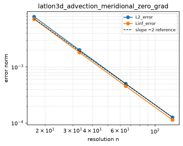
central_D_lev_zero_grad_bc
Source: grids/latlon3d/rules/central_D_lev_zero_grad_bc.esm
Rewrites ∂f/∂lev — match pattern:
{"op": "D", "args": ["f"], "wrt": "lev"}
where): fires only when f is a bare field shaped [lon, lat, lev]. Under import-edge renaming (§9.7.7) the wrt literal and this shape follow the renamed axis together, so the rule can be imported more than once (each instance scoped to its own grid) without a first-declared-wins collision. A consumer differentiating a compound inline expression must bind it to a declared shaped observed first.Discretization — one makearray tiling the output axes; boundary conditions live in the face regions of this same rule (esm-spec §9.6.8; later regions overwrite earlier, §4.3.2):
| Region | Treatment | Value |
|---|---|---|
lon ∈ [1, NLON], lat ∈ [1, NLAT], lev ∈ [2, NLEV−1] | interior | central_D_lev_interior(f)[i,j,k] = ((−(zc[k+1] − zc[k])) / ((zc[k] − zc[k−1])·((zc[k] − zc[k−1]) + (zc[k+1] − zc[k]))))·f[i, j, k−1] + ((zc[k+1] − zc[k] − (zc[k] − zc[k−1])) / ((zc[k] − zc[k−1])·(zc[k+1] − zc[k])))·f[i, j, k] + ((zc[k] − zc[k−1]) / ((zc[k+1] − zc[k])·((zc[k] − zc[k−1]) + (zc[k+1] − zc[k]))))·f[i, j, k+1] for i ∈ lon, j ∈ lat, k ∈ [2, NLEV−1] |
lon ∈ [1, NLON], lat ∈ [1, NLAT], lev = 1 | boundary face | central_D_lev_bottom_face(f)[i,j,k] = ((−(2·(zc[2] − zc[1]) + (zc[3] − zc[2]))) / ((zc[2] − zc[1])·((zc[2] − zc[1]) + (zc[3] − zc[2]))))·f[i, j, 1] + (((zc[2] − zc[1]) + (zc[3] − zc[2])) / ((zc[2] − zc[1])·(zc[3] − zc[2])))·f[i, j, 2] + ((−(zc[2] − zc[1])) / ((zc[3] − zc[2])·((zc[2] − zc[1]) + (zc[3] − zc[2]))))·f[i, j, 3] for i ∈ lon, j ∈ lat, k ∈ [1, 1] |
lon ∈ [1, NLON], lat ∈ [1, NLAT], lev = NLEV | boundary face | central_D_lev_top_face(f)[i,j,k] = ((zc[NLEV] − zc[NLEV−1]) / ((zc[NLEV−1] − zc[NLEV−2])·((zc[NLEV−1] − zc[NLEV−2]) + (zc[NLEV] − zc[NLEV−1]))))·f[i, j, NLEV−2] + ((−((zc[NLEV−1] − zc[NLEV−2]) + (zc[NLEV] − zc[NLEV−1]))) / ((zc[NLEV−1] − zc[NLEV−2])·(zc[NLEV] − zc[NLEV−1])))·f[i, j, NLEV−1] + (((zc[NLEV−1] − zc[NLEV−2]) + 2·(zc[NLEV] − zc[NLEV−1])) / ((zc[NLEV] − zc[NLEV−1])·((zc[NLEV−1] − zc[NLEV−2]) + (zc[NLEV] − zc[NLEV−1]))))·f[i, j, NLEV] for i ∈ lon, j ∈ lat, k ∈ [NLEV, NLEV] |
Centered first derivative along the vertical (lev) axis with zero-gradient (no-flux-compatible) top and bottom boundary levels on the latlon3d grid – the rank-3 vertical analogue of grids/cartesian_nonuniform_1d/rules/central_D1_nonuniform_zero_grad_bc, for vertical advection in a 3-D tracer-transport model such as GEOS-Chem Classic. Matches D(f, wrt: lev). The vertical mesh is NON-UNIFORM (the hybrid sigma-pressure levels): the operator reads the consumer’s level centers zc (shape [lev], defined by applying the grid’s lev_center template to the level-edge array pe) by bare name and uses the exact Fornberg (1988) nonuniform weights, so it is correct on the terrain-following stretched vertical. The body is a makearray tiling [lon, lat, lev] with three regions, each filled by a thin apply of a factored stencil: interior levels [2, NLEV-1] use ../stencils/central_D_lev_interior (3-point centered on zc[k-1..k+1]); the k=1 and k=NLEV boundary levels use ../stencils/central_D_lev_bottom_face and _top_face (second-order one-sided closures on the three nearest centers). ZERO-GRADIENT vs ZERO-FLUX: on a rigid-lid/surface the physical no-flux condition is w=0 at the top and bottom faces, under which the boundary value of this derivative is irrelevant (multiplied by ~0); the zero-gradient one-sided closure is the standard no-flux-compatible treatment and is second-order for a vertically boundary-compatible profile (gradient vanishing at the walls). All three regions are full-rank slab aggregates (output_idx [i,j,k]) so every binding’s simulator fills the (NLON x NLAT x 1) boundary slabs without rank promotion. Second-order in L2 on a smoothly stretched vertical (supraconvergence; see problems/latlon3d_advection_vertical_zero_grad). Match scoping: wrt: lev plus where: {f: {shape: [lon, lat, lev]}} (esm-spec 9.6.1), so it fires only on the vertical derivative of a bare field over THIS grid’s lon x lat x lev index sets; under import renaming (esm-spec 9.7.7) the wrt literal and the where shape follow together. A consumer differentiating a compound inline expression must bind it to a declared lon x lat x lev observed first.
References
- Fornberg, B. (1988). Generation of finite difference formulas on arbitrarily spaced grids. Mathematics of Computation 51(184), 699-706.
doi:10.1090/S0025-5718-1988-0935077-0 - LeVeque, R. J. (2007). Finite Difference Methods for Ordinary and Partial Differential Equations. SIAM. Sections 2.13 (nonuniform grids) and 2.12 (one-sided boundary closures).
Conformance fixtures
- ast:
latlon3d_central_D_lev_zero_grad_bc— statusactive - convergence:
latlon3d_advection_vertical_zero_grad— statusactive - simulation:
latlon3d_advection_3d— statusactive
Convergence — case latlon3d_advection_vertical_zero_grad
Error norms read from the committed golden tests/conformance/convergence/latlon3d_advection_vertical_zero_grad/golden/errors.json (binding: julia; nothing recomputed for display).
| n | L2_error | observed order |
|---|---|---|
| 16 | 2.250e-03 | — |
| 32 | 5.621e-04 | 2.00 |
| 64 | 1.443e-04 | 1.96 |
| 128 | 3.925e-05 | 1.88 |
Expected order: 2 (± 0.25).
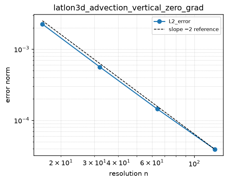
central_D_lon_periodic
Source: grids/latlon3d/rules/central_D_lon_periodic.esm
Rewrites ∂f/∂lon — match pattern:
{"op": "D", "args": ["f"], "wrt": "lon"}
where): fires only when f is a bare field shaped [lon, lat, lev]. Under import-edge renaming (§9.7.7) the wrt literal and this shape follow the renamed axis together, so the rule can be imported more than once (each instance scoped to its own grid) without a first-declared-wins collision. A consumer differentiating a compound inline expression must bind it to a declared shaped observed first.Discretization — one makearray tiling the output axes; boundary conditions live in the face regions of this same rule (esm-spec §9.6.8; later regions overwrite earlier, §4.3.2):
| Region | Treatment | Value |
|---|---|---|
lon ∈ [2, NLON−1], lat ∈ [1, NLAT], lev ∈ [1, NLEV] | interior | central_D_lon_interior(f)[i,j,k] = (f[i+1, j, k] − f[i−1, j, k]) / (2·dlon_deg) for i ∈ [2, NLON−1], j ∈ lat, k ∈ lev |
lon = 1, lat ∈ [1, NLAT], lev ∈ [1, NLEV] | boundary face | (f[2, j, k] − f[NLON, j, k]) / (2·dlon_deg) for i ∈ [1, 1], j ∈ lat, k ∈ lev |
lon = NLON, lat ∈ [1, NLAT], lev ∈ [1, NLEV] | boundary face | (f[1, j, k] − f[NLON−1, j, k]) / (2·dlon_deg) for i ∈ [NLON, NLON], j ∈ lat, k ∈ lev |
Centered first derivative along longitude with a periodic (wrap) boundary on the latlon3d grid — the rank-3 (lon x lat x lev) extension of grids/latlon/rules/central_D_lon_periodic and the zonal sibling of ./central_D_lat_zero_grad_bc. Matches D(f, wrt: lon), a PER-DEGREE derivative. THE NON-UPWIND ZONAL DERIVATIVE ON THIS GRID: unlike the transport rules ppm_flux_D_lon_mono_periodic / upwind1_D_lon_periodic, it carries no velocity and no donor-cell bias, so it is the right operator for a term that is a plain gradient rather than an advective flux — the zonal PRESSURE-GRADIENT FORCE of a hydrostatic dynamical core being the motivating consumer (a centred, non-dissipative gradient is what keeps geostrophic balance from being damped). Interior columns [2, NLON-1] use the imported ../stencils/central_D_lon_interior. The two face columns wrap explicitly, following the rank-2 sibling and the cartesian upwind1_D_periodic precedent: i=1 gathers (f[2,j,k] - f[NLON,j,k]) / (2 dlon_deg) and i=NLON gathers (f[1,j,k] - f[NLON-1,j,k]) / (2 dlon_deg), so the scheme is the same O(dlon_deg^2) centered difference at every column and conserves sum(f) exactly (the wrap telescopes). The face values are FULL-RANK aggregates (singleton output range on the lon axis) rather than the esm-spec 9.6.8 worked example’s rank-reduced form, so every binding’s simulator fills the (1 x NLAT x NLEV) regions without rank promotion. dlon_deg is a free name resolving to the consuming model’s zonal spacing variable; the rule itself never assumes the global extent, but composing it with a non-closing regional grid is a modeling error. Match scoping: the pattern is wrt: lon plus the constraint where: {f: {shape: [lon, lat, lev]}} (esm-spec 9.6.1), so it fires only on the longitudinal derivative of a bare field declared over this grid’s lon x lat x lev index sets, and under import-edge renaming (esm-spec 9.7.7) the wrt literal and the where shape follow the renamed axis together. The constraint requires a bare declared shaped field — a consumer differentiating a compound inline expression must bind it to a declared lon x lat x lev observed first (which is also how a rank-2 surface field such as log surface pressure is differentiated here: broadcast it to rank 3 and declare that observed).
References
- LeVeque, R. J. (2007). Finite Difference Methods for Ordinary and Partial Differential Equations. SIAM. Section 10.4 (centered differences on periodic domains).
Conformance fixtures
- ast:
central_D_lon_periodic— statusactive - ast:
latlon3d_central_D_lon_periodic— statusactive - convergence:
latlon3d_advection_zonal_central— statusactive
Convergence — case latlon3d_advection_zonal_central
Error norms read from the committed golden tests/conformance/convergence/latlon3d_advection_zonal_central/golden/errors.json (binding: julia; nothing recomputed for display).
| n | L2_error | observed order | Linf_error | observed order |
|---|---|---|---|---|
| 16 | 2.003e-02 | — | 1.968e-02 | — |
| 32 | 5.037e-03 | 1.99 | 5.014e-03 | 1.97 |
| 64 | 1.261e-03 | 2.00 | 1.260e-03 | 1.99 |
| 128 | 3.154e-04 | 2.00 | 3.153e-04 | 2.00 |
Expected order: 2 (± 0.2).
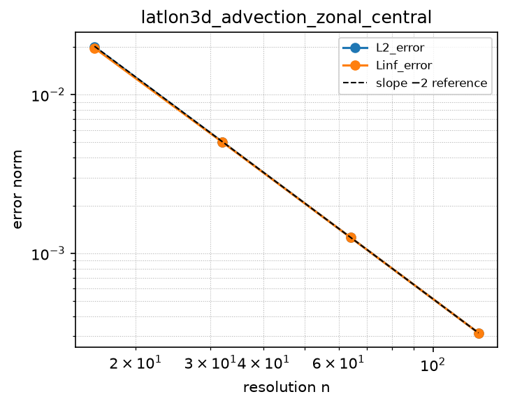
face_flux_divergence_lat_open_bc
Source: grids/latlon3d/rules/face_flux_divergence_lat_open_bc.esm
Rewrites ∂My/∂lat at priority 10 — match pattern:
{"op": "D", "args": ["My"], "wrt": "lat"}
where): fires only when My is a bare field shaped [lon, lat_nodes, lev]. Under import-edge renaming (§9.7.7) the wrt literal and this shape follow the renamed axis together, so the rule can be imported more than once (each instance scoped to its own grid) without a first-declared-wins collision. A consumer differentiating a compound inline expression must bind it to a declared shaped observed first.Discretization — one makearray tiling the output axes; boundary conditions live in the face regions of this same rule (esm-spec §9.6.8; later regions overwrite earlier, §4.3.2):
| Region | Treatment | Value |
|---|---|---|
lon ∈ [1, NLON], lat ∈ [1, NLAT], lev ∈ [1, NLEV] | interior | facediv_lat_open_interior(My)[i,j,k] = (My[i, j+1, k]·coslat_e[j+1] − My[i, j, k]·coslat_e[j]) / dS_lat[j] for i ∈ lon, j ∈ [1, NLAT], k ∈ lev |
OPEN-WALL (regional limited-area) MERIDIONAL continuity D(My, wrt: lat) on latlon3d: the air-mass half of a consistency-with-continuity pair whose tracer half is rules/ppm_flux_D_lat_mono_inflow_bc. A regional model writes d(m)/dt = -D(My, wrt: lat) + … for the air mass m and the face air-mass flux My, alongside d(mq)/dt = -D(My*q, wrt: lat) for the tracer; a constant q is preserved bitwise because the PPM flux collapses to My at every face – INCLUDING the open walls – when the boundary halo is uniform. The open-boundary sibling of face_flux_divergence_lat_polar: same metric, same face convention, but the wall faces are DIFFERENCED (real open boundary) rather than omitted at the poles. A single full-axis region applies ../stencils/facediv_lat_open_interior. Match D(My, wrt: lat) at priority 10 with a where-shape constraint marking My as the face-staggered flux over [’lon’, ’lat_nodes’, ’lev’]; a consuming problem imports exactly one lat continuity rule. Semi-discrete (method-of-lines). Requires NLAT >= 1.
References
- Lin, S.-J., & Rood, R. B. (1996). Multidimensional flux-form semi-Lagrangian transport schemes. Monthly Weather Review, 124(9), 2046-2070.
doi:10.1175/1520-0493(1996)124<2046:MFFSLT>2.0.CO;2 - Jockel, P., von Kuhlmann, R., Lawrence, M. G., et al. (2001). On a fundamental problem in implementing flux-form advection schemes for tracer transport in 3-dimensional general circulation and chemistry transport models. Quarterly Journal of the Royal Meteorological Society, 127(573), 1035-1052.
doi:10.1002/qj.49712757318 - Jacobson, M. Z. (2005). Fundamentals of Atmospheric Modeling (2nd ed.). Cambridge University Press. Chapter 6 (finite-volume flux-form tracer transport; consistency with continuity).
Conformance fixtures
- simulation:
latlon3d_transport_cwc_regional_inflow - simulation:
latlon3d_transport_per_tracer_inflow
face_flux_divergence_lat_polar
Source: grids/latlon3d/rules/face_flux_divergence_lat_polar.esm
Rewrites ∂My/∂lat at priority 10 — match pattern:
{"op": "D", "args": ["My"], "wrt": "lat"}
where): fires only when My is a bare field shaped [lon, lat_nodes, lev]. Under import-edge renaming (§9.7.7) the wrt literal and this shape follow the renamed axis together, so the rule can be imported more than once (each instance scoped to its own grid) without a first-declared-wins collision. A consumer differentiating a compound inline expression must bind it to a declared shaped observed first.Discretization — one makearray tiling the output axes; boundary conditions live in the face regions of this same rule (esm-spec §9.6.8; later regions overwrite earlier, §4.3.2):
| Region | Treatment | Value |
|---|---|---|
lon ∈ [1, NLON], lat ∈ [2, NLAT−1], lev ∈ [1, NLEV] | interior | facediv_lat_interior(My)[i,j,k] = (My[i, j+1, k]·coslat_e[j+1] − My[i, j, k]·coslat_e[j]) / dS_lat[j] for i ∈ lon, j ∈ [2, NLAT−1], k ∈ lev |
lon ∈ [1, NLON], lat = 1, lev ∈ [1, NLEV] | boundary face | facediv_lat_cap_s(My)[i,j,k] = (My[i, 2, k]·coslat_e[2]) / dS_lat[1] for i ∈ lon, j ∈ [1, 1], k ∈ lev |
lon ∈ [1, NLON], lat = NLAT, lev ∈ [1, NLEV] | boundary face | facediv_lat_cap_n(My)[i,j,k] = (−(My[i, NLAT, k]·coslat_e[NLAT])) / dS_lat[NLAT] for i ∈ lon, j ∈ [NLAT, NLAT], k ∈ lev |
MERIDIONAL DIVERGENCE OF A FACE-STAGGERED FLUX on the latlon3d spherical grid, (1/(a cos phi)) d/dphi ( cos(phi) My ), with the pole treated as a ZERO-LENGTH FACE (no flux) at both ends. The consuming model writes its CONTINUITY equation as d(m)/dt = -D(My, wrt: lat), where m is the air mass per unit area in the cell (shape [lon, lat, lev]) and My is the face-staggered northward air-mass flux (shape [lon, lat_nodes, lev]). This is the exact MERIDIONAL TWIN of face_flux_divergence_lev_noflux_bc, and the continuity companion of the flux-form advection rule upwind1_flux_D_lat_polar.
WHAT THE OPERATOR IS. In index form D[i,j,k] = ( My[i,j+1,k] coslat_e[j+1] - My[i,j,k] coslat_e[j] ) / dS_lat[j] on the interior rows, with the two POLE terms structurally omitted: D[i,1,k] = My[i,2,k] coslat_e[2] / dS_lat[1] and D[i,NLAT,k] = -My[i,NLAT,k] coslat_e[NLAT] / dS_lat[NLAT]. coslat_e is the FACE-LENGTH weight cos(phi_e) on the lat_nodes axis and dS_lat the EXACT spherical cell-AREA weight sin(phi_e[j+1]) - sin(phi_e[j]) on the lat axis; both are read as FREE NAMES from the consuming model’s scope – the same contract by which the vertical rules read dz – and the consumer builds them from the grid templates: an observed phie = lat_edge() of shape [lat_nodes], then coslat_e = coslat_edge(phie) and dS_lat = latcell_area(phie).
WHY IT EXISTS: CONSISTENCY WITH CONTINUITY. The flux-form advection rule upwind1_flux_D_lat_polar transports a MIXING RATIO with a PRESCRIBED wind: d(u)/dt = -D(Vu, wrt: lat). That is mass-conservative in u, but it is NOT free-stream preserving – set u == 1 and the right-hand side becomes the discrete divergence of the wind itself, which is nonzero wherever the flow diverges, so a uniform tracer spontaneously develops structure out of nothing. The physical error is that a mixing ratio is a ratio to a mass the model never carried. The fix is to carry it: evolve the air mass m with THIS rule, evolve the tracer mass mq with the advection rule applied to the compound D(Myq, wrt: lat), and define the mixing ratio as the observed q = mq/m. A constant q is then preserved, because the tracer equation reduces term-by-term to the mass equation – the property Jockel et al. (2001) call consistency with continuity, and the one Lin & Rood (1996) enforce by construction by having the tracer scheme reuse the continuity scheme’s mass fluxes.
AND IT IS PRESERVED BITWISE, NOT MERELY TO ROUNDING. With q == 1 the donor-cell face flux of the advection rule, F = 1/2[My(qL + qR) - |My|(qR - qL)], collapses to 1/2[My*2 - |My|0] = My – and every step of that collapse is EXACT in IEEE binary floating point (1+1 = 2 exactly, My2 exactly, 1-1 = 0 exactly, |My|0 = 0 exactly, 0.5(2My) = My exactly). This rule and the advection rule then apply the IDENTICAL remaining operations in the IDENTICAL order – the same face pairing, the same coslat_e face-length factors, the same dS_lat divisor, the same unary negation at the north cap – so the tracer divergence emits, cell by cell, the identical double-precision numbers this rule emits, mq stays bit-for-bit equal to m through every Runge-Kutta stage, and q = mq/m evaluates to exactly 1.0 (IEEE division of a value by itself). Measured max|q - 1| over a trajectory under a strongly divergent meridional mass flux: 0.0, not 1e-16.
THE POLE OMISSION IS LOAD-BEARING FOR THAT EXACTNESS. Both rules DELETE the pole-wall terms rather than forming them and multiplying by the pole face length – which on the global recipe is cos(-/+pi/2) = 6.1e-17 in IEEE double, NOT zero. Had one family formed its wall term and the other omitted it, the two would agree only to rounding, the meridional mass budget would leak, and a constant tracer would acquire structure at the caps. The same omission is what makes the operator EXACTLY conservative: sum_j dS_lat[j] D[i,j,k] telescopes to zero, since every interior face term appears once with each sign and neither pole term is ever formed.
HOW IT IS SEPARATED FROM THE PLAIN-D LAT RULES, AND WHY THAT SEPARATION IS STRUCTURAL. The match pattern is a BARE derivative D(My, wrt: lat) – structurally the same pattern as the pre-existing plain-D lat rules on this grid (central_D_lat_zero_grad_bc, ppm_D_lat_zero_grad_bc). What separates them is the esm-spec 9.6.1 where SHAPE CONSTRAINT, not priority: those rules constrain their operand to [lon, lat, lev] (cell centres) and this one to [lon, lat_nodes, lev] (the NLAT+1 face axis), and no declared field can satisfy both. It is likewise disjoint from the flux-form advection rule, whose pattern requires the operand to be a two-factor PRODUCT: D(Myq, wrt: lat) does not match a bare D(My, wrt: lat), and conversely this rule cannot capture D(Myq) because a shape constraint is satisfied only by a bare variable-reference string and never by a compound sub-AST. The three rules – mass divergence, tracer flux divergence, cell-centred derivative – coexist in a single model, each firing on its own term.
EXACTNESS AND THE ORDER TAG. Read as a finite-volume operator on cell MEANS, this operator has NO truncation error: the integral of d/dphi(cos(phi) My) over the cell is exactly the difference of cos(phi) My at the two bounding edges (fundamental theorem of calculus), and dS_lat is the EXACT area weight, not a midpoint approximation. Given exact face fluxes the discrete continuity equation is therefore solved exactly at every resolution, INCLUDING at the polar caps – the O(dphi/cos(phi)) accuracy story that governs the ADVECTION rule (see its ACCURACY AT THE POLES section) does not arise here, because there is no reconstruction to be inaccurate. The order:1 tag is the conservative POINTWISE claim, following the convention of face_flux_divergence_lev_noflux_bc and grids/mpas/rules/fv_divergence_cell. Requires NLAT >= 3.
References
- Jockel, P., von Kuhlmann, R., Lawrence, M. G., et al. (2001). On a fundamental problem in implementing flux-form advection schemes for tracer transport in 3-dimensional general circulation and chemistry transport models. Quarterly Journal of the Royal Meteorological Society, 127(573), 1035-1052. (Consistency with continuity: what breaks when the tracer scheme and the continuity scheme do not use the same mass fluxes.)
doi:10.1002/qj.49712757318 - Lin, S.-J., & Rood, R. B. (1996). Multidimensional flux-form semi-Lagrangian transport schemes. Monthly Weather Review, 124(9), 2046-2070.
doi:10.1175/1520-0493(1996)124<2046:MFFSLT>2.0.CO;2 - LeVeque, R. J. (2002). Finite Volume Methods for Hyperbolic Problems. Cambridge University Press. Section 4.1 (the finite-volume divergence as a telescoping difference of face fluxes).
- Jacobson, M. Z. (2005). Fundamentals of Atmospheric Modeling (2nd ed.). Cambridge University Press. Chapter 6.
Conformance fixtures
- ast:
latlon3d_face_flux_divergence_lat_polar— statusactive - simulation:
latlon3d_transport_cwc_3d— statusactive - simulation:
latlon3d_transport_cwc_3d_ppm
face_flux_divergence_lev_massform_noflux_bc
Source: grids/latlon3d/rules/face_flux_divergence_lev_massform_noflux_bc.esm
Rewrites ∂M/∂lev at priority 10 — match pattern:
{"op": "D", "args": ["M"], "wrt": "lev"}
where): fires only when M is a bare field shaped [lon, lat, lev_nodes]. Under import-edge renaming (§9.7.7) the wrt literal and this shape follow the renamed axis together, so the rule can be imported more than once (each instance scoped to its own grid) without a first-declared-wins collision. A consumer differentiating a compound inline expression must bind it to a declared shaped observed first.Discretization — one makearray tiling the output axes; boundary conditions live in the face regions of this same rule (esm-spec §9.6.8; later regions overwrite earlier, §4.3.2):
| Region | Treatment | Value |
|---|---|---|
lon ∈ [1, NLON], lat ∈ [1, NLAT], lev ∈ [2, NLEV−1] | interior | facediv_lev_mass_interior(M)[i,j,k] = M[i, j, k+1] − M[i, j, k] for i ∈ lon, j ∈ lat, k ∈ [2, NLEV−1] |
lon ∈ [1, NLON], lat ∈ [1, NLAT], lev = 1 | boundary face | facediv_lev_mass_nf_k1(M)[i,j,k] = M[i, j, 2] for i ∈ lon, j ∈ lat, k ∈ [1, 1] |
lon ∈ [1, NLON], lat ∈ [1, NLAT], lev = NLEV | boundary face | facediv_lev_mass_nf_kN(M)[i,j,k] = −M[i, j, NLEV] for i ∈ lon, j ∈ lat, k ∈ [NLEV, NLEV] |
MASS-FORM vertical DIVERGENCE OF A FACE-STAGGERED FLUX, the moving-grid continuity companion for a TERRAIN-FOLLOWING (hybrid sigma-pressure) vertical coordinate. The consumer writes its air-mass continuity as ddp/dt = -D(M, wrt: lev) + … where dp is the cell air mass per unit area (the pressure thickness, shape [lon,lat,lev]) and M is the vertical air-mass flux (shape [lon,lat,lev_nodes], positive upward). Unlike its FIXED-GRID sibling face_flux_divergence_lev_noflux_bc, which returns (M_{k+1/2}-M_{k-1/2})/dz[k], this returns the RAW difference M_{k+1/2}-M_{k-1/2} with no thickness division: dividing by a time-varying dz omits the grid-motion term and is conservative only on a fixed grid, whereas the raw flux difference integrates the extensive cell mass directly and stays conservative while the layers breathe. It is the EXACT q == 1 limit of the terrain-following advection rule ppm_flux_D_lev_mono_hybrid_noflux_bc, so a tracer initialised to a uniform mixing ratio tracks the breathing air mass to the last bit – the consistency-with-continuity property verified by tests/conformance/simulation/latlon3d_transport_cwc_moving_lid. Three regions (interior k=2..NLEV-1, ground k=1, model top k=NLEV) with rigid no-flux walls; M at faces 1 and NLEV+1 is never read.
References
- Jockel, P., von Kuhlmann, R., Lawrence, M. G., et al. (2001). On a fundamental problem in implementing flux-form advection schemes for tracer transport in 3-dimensional general circulation and chemistry transport models. Quarterly Journal of the Royal Meteorological Society, 127(573), 1035-1052. (Consistency with continuity: what breaks when the tracer scheme and the continuity scheme do not use the same mass fluxes.)
doi:10.1002/qj.49712757318 - Lin, S.-J., & Rood, R. B. (1996). Multidimensional flux-form semi-Lagrangian transport schemes. Monthly Weather Review, 124(9), 2046-2070.
doi:10.1175/1520-0493(1996)124<2046:MFFSLT>2.0.CO;2 - LeVeque, R. J. (2002). Finite Volume Methods for Hyperbolic Problems. Cambridge University Press. Section 4.1 (the finite-volume divergence as a telescoping difference of face fluxes).
- Jacobson, M. Z. (2005). Fundamentals of Atmospheric Modeling (2nd ed.). Cambridge University Press. Chapter 6.
Conformance fixtures
- ast:
latlon3d_face_flux_divergence_lev_massform_noflux_bc— statusactive - simulation:
latlon3d_transport_cwc_moving_lid
face_flux_divergence_lev_noflux_bc
Source: grids/latlon3d/rules/face_flux_divergence_lev_noflux_bc.esm
Rewrites ∂M/∂lev at priority 10 — match pattern:
{"op": "D", "args": ["M"], "wrt": "lev"}
where): fires only when M is a bare field shaped [lon, lat, lev_nodes]. Under import-edge renaming (§9.7.7) the wrt literal and this shape follow the renamed axis together, so the rule can be imported more than once (each instance scoped to its own grid) without a first-declared-wins collision. A consumer differentiating a compound inline expression must bind it to a declared shaped observed first.Discretization — one makearray tiling the output axes; boundary conditions live in the face regions of this same rule (esm-spec §9.6.8; later regions overwrite earlier, §4.3.2):
| Region | Treatment | Value |
|---|---|---|
lon ∈ [1, NLON], lat ∈ [1, NLAT], lev ∈ [2, NLEV−1] | interior | facediv_lev_interior(M)[i,j,k] = (M[i, j, k+1] − M[i, j, k]) / dz[k] for i ∈ lon, j ∈ lat, k ∈ [2, NLEV−1] |
lon ∈ [1, NLON], lat ∈ [1, NLAT], lev = 1 | boundary face | facediv_lev_nf_k1(M)[i,j,k] = M[i, j, 2] / dz[1] for i ∈ lon, j ∈ lat, k ∈ [1, 1] |
lon ∈ [1, NLON], lat ∈ [1, NLAT], lev = NLEV | boundary face | facediv_lev_nf_kN(M)[i,j,k] = (−M[i, j, NLEV]) / dz[NLEV] for i ∈ lon, j ∈ lat, k ∈ [NLEV, NLEV] |
Vertical DIVERGENCE OF A FACE-STAGGERED FLUX, d/dz(M), on the latlon3d non-uniform vertical, with rigid NO-FLUX walls at the surface and the model top. The consuming model writes its CONTINUITY equation as d(m)/dt = -D(M, wrt: lev), where m is the air mass per unit area in the cell (the pressure thickness dp, shape [lon, lat, lev]) and M is the face air-mass flux (shape [lon, lat, lev_nodes], positive upward). Assembled from three region stencils – facediv_lev_interior (k = 2..NLEV-1), facediv_lev_nf_k1 (the ground) and facediv_lev_nf_kN (the lid) – exactly mirroring the region structure of upwind1_flux_D_lev_noflux_bc, which is what makes the pair consistent.
WHY IT EXISTS: CONSISTENCY WITH CONTINUITY. The flux-form advection rule upwind1_flux_D_lev_noflux_bc transports a MIXING RATIO with a PRESCRIBED wind: d(u)/dt = -D(Wu, wrt: lev). That is mass-conservative in u, but it is NOT free-stream preserving – set u == 1 and the right-hand side becomes -dW/dz, which is nonzero wherever the wind diverges, so a uniform tracer spontaneously develops structure out of nothing. The physical error is that a mixing ratio is a ratio to a mass that the model never carried. The fix is to carry it: evolve the air mass m with THIS rule, evolve the tracer mass mq with the advection rule applied to the compound D(Mq, wrt: lev), and define the mixing ratio as the observed q = mq/m. Then a constant q is preserved, because the tracer equation reduces term-by-term to the mass equation. This is the property Jockel et al. (2001) call consistency with continuity, and the one Lin & Rood (1996) enforce by construction by having the tracer scheme reuse the continuity scheme’s mass fluxes.
AND IT IS PRESERVED BITWISE, NOT MERELY TO ROUNDING. With q == 1 the donor-cell face flux of the advection rule, F = 1/2[w(qL + qR) - |w|(qR - qL)], collapses to 1/2[M*2 - |M|0] = M – and every step of that collapse is EXACT in IEEE binary floating point (1+1 = 2 exactly, M2 exactly, 1-1 = 0 exactly, |M|0 = 0 exactly, 0.5(2M) = M exactly). The tracer divergence therefore emits, cell by cell, the identical double-precision numbers this rule emits, mq stays bit-for-bit equal to m through every Runge-Kutta stage, and q = mq/m evaluates to exactly 1.0 (IEEE division of a value by itself). The measured max|q - 1| over a trajectory under a strongly divergent wind is 0.0, not 1e-16. That exactness is not an accident of the algebra alone: it requires the two rules to difference the SAME faces with the SAME thicknesses and, critically, to OMIT the wall fluxes in the same way – which is why both families write the no-flux closure by literally deleting the wall term rather than by forming it and multiplying by zero.
HOW IT IS SEPARATED FROM THE PLAIN-D RULES, AND WHY THAT SEPARATION IS STRUCTURAL. The match pattern is a BARE derivative D(M, wrt: lev) – structurally the same pattern as the pre-existing plain-D lev rules on this grid (central_D_lev_zero_grad_bc, ppm_D_lev_noflux_bc, ppm_D_lev_mono_noflux_bc). What separates them is the esm-spec 9.6.1 where SHAPE CONSTRAINT, not priority: those rules constrain their operand to [lon, lat, lev] (cell centres) and this one to [lon, lat, lev_nodes] (the NLEV+1 face axis), and no declared field can satisfy both. A model may therefore import this rule alongside any of them – a plain D(q, wrt: lev) on a cell-centred tracer still lowers to the cell-centred rule, and a D(M, wrt: lev) on a face-staggered flux lowers here – with no ambiguity and no priority race. It is likewise disjoint from the flux-form advection rule, whose pattern requires the operand to be a two-factor PRODUCT: D(Mq, wrt: lev) does not match a bare D(M, wrt: lev), and conversely this rule cannot capture D(Mq) because a shape constraint is satisfied only by a bare variable reference and never by a compound sub-AST. The three rules – mass divergence, tracer flux divergence, cell-centred derivative – coexist in a single model, each firing on its own term.
EXACTNESS AND THE ORDER TAG. Read as a finite-volume operator on cell MEANS, this operator has NO truncation error: the cell mean of dM/dz is the difference of the exact face fluxes over the thickness, identically. Given exact face fluxes the discrete continuity equation is therefore solved exactly at every resolution (a free-running m evolves as its exact cell average), and the column mass sum telescopes to the two wall fluxes – both zero – so total air mass is conserved to the last bit. The order:1 tag is the conservative POINTWISE claim (second order as an approximation to dM/dz at the cell centre on a uniform mesh, first order on a stretched one), following the convention of grids/mpas/rules/fv_divergence_cell. Requires NLEV >= 3.
References
- Jockel, P., von Kuhlmann, R., Lawrence, M. G., et al. (2001). On a fundamental problem in implementing flux-form advection schemes for tracer transport in 3-dimensional general circulation and chemistry transport models. Quarterly Journal of the Royal Meteorological Society, 127(573), 1035-1052. (Consistency with continuity: what breaks when the tracer scheme and the continuity scheme do not use the same mass fluxes.)
doi:10.1002/qj.49712757318 - Lin, S.-J., & Rood, R. B. (1996). Multidimensional flux-form semi-Lagrangian transport schemes. Monthly Weather Review, 124(9), 2046-2070.
doi:10.1175/1520-0493(1996)124<2046:MFFSLT>2.0.CO;2 - LeVeque, R. J. (2002). Finite Volume Methods for Hyperbolic Problems. Cambridge University Press. Section 4.1 (the finite-volume divergence as a telescoping difference of face fluxes).
- Jacobson, M. Z. (2005). Fundamentals of Atmospheric Modeling (2nd ed.). Cambridge University Press. Chapter 6.
Conformance fixtures
- ast:
latlon3d_face_flux_divergence_lev_noflux_bc— statusactive - convergence:
latlon3d_transport_cwc_mms— statusactive - simulation:
latlon3d_transport_cwc_3d— statusactive - simulation:
latlon3d_transport_cwc_3d_ppm
Convergence — case latlon3d_transport_cwc_mms
Error norms read from the committed golden tests/conformance/convergence/latlon3d_transport_cwc_mms/golden/errors.json (binding: julia; nothing recomputed for display).
| n | L2_error | observed order | Linf_error | observed order |
|---|---|---|---|---|
| 32 | 2.169e-03 | — | 1.694e-02 | — |
| 64 | 1.092e-03 | 0.99 | 9.106e-03 | 0.90 |
| 128 | 5.480e-04 | 1.00 | 4.715e-03 | 0.95 |
| 256 | 2.747e-04 | 1.00 | 2.399e-03 | 0.98 |
Expected order: 1 (± 0.15).
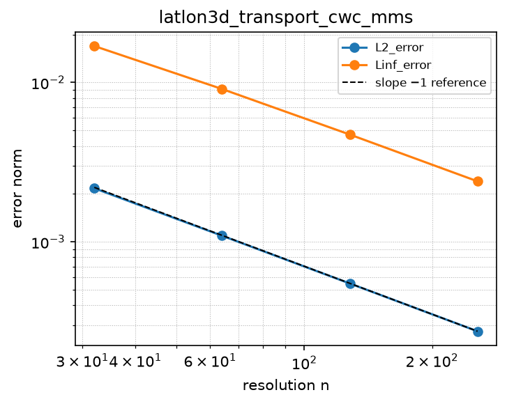
face_flux_divergence_lon_open_bc
Source: grids/latlon3d/rules/face_flux_divergence_lon_open_bc.esm
Rewrites ∂Mx/∂lon at priority 10 — match pattern:
{"op": "D", "args": ["Mx"], "wrt": "lon"}
where): fires only when Mx is a bare field shaped [lon_nodes, lat, lev]. Under import-edge renaming (§9.7.7) the wrt literal and this shape follow the renamed axis together, so the rule can be imported more than once (each instance scoped to its own grid) without a first-declared-wins collision. A consumer differentiating a compound inline expression must bind it to a declared shaped observed first.Discretization — one makearray tiling the output axes; boundary conditions live in the face regions of this same rule (esm-spec §9.6.8; later regions overwrite earlier, §4.3.2):
| Region | Treatment | Value |
|---|---|---|
lon ∈ [1, NLON], lat ∈ [1, NLAT], lev ∈ [1, NLEV] | interior | facediv_lon_open_interior(Mx)[i,j,k] = (dphi_lat[j] / ((dlon_deg·(3.14159265359 / 180))·dS_lat[j]))·(Mx[i+1, j, k] − Mx[i, j, k]) for i ∈ [1, NLON], j ∈ lat, k ∈ lev |
OPEN-WALL (regional limited-area) ZONAL continuity D(Mx, wrt: lon) on latlon3d: the air-mass half of a consistency-with-continuity pair whose tracer half is rules/ppm_flux_D_lon_mono_inflow_bc. A regional model writes d(m)/dt = -D(Mx, wrt: lon) + … for the air mass m and the face air-mass flux Mx, alongside d(mq)/dt = -D(Mx*q, wrt: lon) for the tracer; a constant q is preserved bitwise because the PPM flux collapses to Mx at every face – INCLUDING the open walls – when the boundary halo is uniform. The open-boundary sibling of face_flux_divergence_lon_periodic: same metric, same face convention, but the wall faces are DIFFERENCED (real open boundary) rather than wrapped around the zonal circle. A single full-axis region applies ../stencils/facediv_lon_open_interior. Match D(Mx, wrt: lon) at priority 10 with a where-shape constraint marking Mx as the face-staggered flux over [’lon_nodes’, ’lat’, ’lev’]; a consuming problem imports exactly one lon continuity rule. Semi-discrete (method-of-lines). Requires NLON >= 1.
References
- Lin, S.-J., & Rood, R. B. (1996). Multidimensional flux-form semi-Lagrangian transport schemes. Monthly Weather Review, 124(9), 2046-2070.
doi:10.1175/1520-0493(1996)124<2046:MFFSLT>2.0.CO;2 - Jockel, P., von Kuhlmann, R., Lawrence, M. G., et al. (2001). On a fundamental problem in implementing flux-form advection schemes for tracer transport in 3-dimensional general circulation and chemistry transport models. Quarterly Journal of the Royal Meteorological Society, 127(573), 1035-1052.
doi:10.1002/qj.49712757318 - Jacobson, M. Z. (2005). Fundamentals of Atmospheric Modeling (2nd ed.). Cambridge University Press. Chapter 6 (finite-volume flux-form tracer transport; consistency with continuity).
Conformance fixtures
- simulation:
latlon3d_transport_cwc_regional_inflow - simulation:
latlon3d_transport_per_tracer_inflow
face_flux_divergence_lon_periodic
Source: grids/latlon3d/rules/face_flux_divergence_lon_periodic.esm
Rewrites ∂Mx/∂lon at priority 10 — match pattern:
{"op": "D", "args": ["Mx"], "wrt": "lon"}
where): fires only when Mx is a bare field shaped [lon_nodes, lat, lev]. Under import-edge renaming (§9.7.7) the wrt literal and this shape follow the renamed axis together, so the rule can be imported more than once (each instance scoped to its own grid) without a first-declared-wins collision. A consumer differentiating a compound inline expression must bind it to a declared shaped observed first.Discretization — one makearray tiling the output axes; boundary conditions live in the face regions of this same rule (esm-spec §9.6.8; later regions overwrite earlier, §4.3.2):
| Region | Treatment | Value |
|---|---|---|
lon ∈ [1, NLON−1], lat ∈ [1, NLAT], lev ∈ [1, NLEV] | interior | facediv_lon_interior(Mx)[i,j,k] = (dphi_lat[j] / ((dlon_deg·(3.14159265359 / 180))·dS_lat[j]))·(Mx[i+1, j, k] − Mx[i, j, k]) for i ∈ [1, NLON−1], j ∈ lat, k ∈ lev |
lon = NLON, lat ∈ [1, NLAT], lev ∈ [1, NLEV] | boundary face | facediv_lon_wrap_iN(Mx)[i,j,k] = (dphi_lat[j] / ((dlon_deg·(3.14159265359 / 180))·dS_lat[j]))·(Mx[1, j, k] − Mx[NLON, j, k]) for i ∈ [NLON, NLON], j ∈ lat, k ∈ lev |
ZONAL DIVERGENCE OF A FACE-STAGGERED FLUX, D(Mx, wrt: lon), on the latlon3d grid, with the PERIODIC WRAP ENFORCED INSIDE THE RULE. The consuming model writes its CONTINUITY equation as dm/dt = -D(Mx, wrt: lon) + …, where m is the air mass per unit area in the cell (shape [lon, lat, lev]) and Mx the face air-mass flux (shape [lon_nodes, lat, lev], positive eastward). It is the CONTINUITY COMPANION of upwind1_flux_D_lon_periodic and the zonal sibling of face_flux_divergence_lev_noflux_bc. In index form D[i,j,k] = ( dphi_lat[j] / (dlam dS_lat[j]) ) ( Mx[i+1,j,k] - Mx[i,j,k] ), with dlam = dlon_deg pi/180 and the SAME wrap as the advection rule: at i = NLON the upper face value is Mx[1], NEVER Mx[NLON+1]. Assembled from two region stencils – facediv_lon_interior (i = 1 .. NLON-1) and facediv_lon_wrap_iN – and Mx[NLON+1,j,k] is consequently NEVER READ.
WHY IT EXISTS: CONSISTENCY WITH CONTINUITY, AND WHY IT MUST BE EXACT. The flux-form advection rule transports a MIXING RATIO with a PRESCRIBED wind: du/dt = -D(Uu, wrt: lon). That is mass-conservative in u, but not free-stream preserving – set u == 1 and the right-hand side becomes -dU/dlam (times the metric), which is nonzero wherever the wind converges, so a uniform tracer spontaneously develops structure out of nothing. The physical error is that a mixing ratio is a ratio to a mass the model never carried. The fix is to carry it: evolve the air mass m with THIS rule, the tracer mass mq with the advection rule applied to D(Mxq, wrt: lon), and define q = mq/m. Then a constant q is preserved, because the tracer equation reduces term-by-term to the mass equation – what Jockel et al. (2001) call consistency with continuity, and what Lin & Rood (1996) enforce by construction by having the tracer scheme reuse the continuity scheme’s mass fluxes.
AND IT IS PRESERVED BITWISE, NOT MERELY TO ROUNDING. With q == 1 the donor-cell face flux of the advection rule, F = 1/2[w(qL + qR) - |w|(qR - qL)], collapses to 1/2[Mx2 - |Mx|0] = Mx – and every step of that collapse is EXACT in IEEE binary floating point (1+1 = 2 exactly, Mx2 exactly, 1-1 = 0 exactly, |Mx|0 = 0 exactly, 0.5(2 Mx) = Mx exactly). Because this rule differences the SAME faces, WRAPS IN THE SAME PLACE, and multiplies by the SAME metric weight – spelled as the same op tree with the same literals – D(U1, wrt: lon) is bit-for-bit D(Mx, wrt: lon) evaluated at Mx := U. MEASURED: 0 ulp on every element, i.e. the two arrays are === identical, not equal to 1e-16. Get the two rules out of step about ANY face, ANY weight or THE WRAP and free-stream preservation breaks silently.
HOW IT IS SEPARATED FROM THE PLAIN-D LON RULES, AND WHY THAT SEPARATION IS STRUCTURAL. The match pattern is a BARE derivative D(Mx, wrt: lon) – structurally the same pattern as the pre-existing plain-D lon rules on this grid (upwind1_D_lon_periodic, ppm_D_lon_periodic). What separates them is the esm-spec 9.6.1 where SHAPE CONSTRAINT, not priority: those rules constrain their operand to [lon, lat, lev] (cell centres) and this one to [lon_nodes, lat, lev] (the NLON+1 face axis), and no declared field can satisfy both. A model may therefore import this rule alongside any of them with no ambiguity and no priority race. It is likewise disjoint from the flux-form advection rule, whose pattern requires the operand to be a two-factor PRODUCT: D(Mxq, wrt: lon) does not match a bare D(Mx, wrt: lon), and conversely this rule cannot capture D(Mxq) because a shape constraint is satisfied only by a bare variable reference and never by a compound sub-AST.
EXACTNESS AND THE ORDER TAG. Read as a finite-volume operator on cell MEANS, this operator has NO truncation error: the cell mean of the zonal flux divergence is the difference of the exact face fluxes times dphi_lat/(dlam dS_lat), identically. Given exact face fluxes the discrete continuity equation is solved exactly at every resolution, and the wrap makes the two boundary terms of the zonal sum cancel BIT-FOR-BIT (both are Mx[1]), so the row-summed air-mass budget is zero to machine precision – measured max |sum_i D| = 5.0e-15 – for any Mx, periodic or not. The order:1 tag is the conservative POINTWISE claim, following the convention of grids/mpas/rules/fv_divergence_cell and the vertical sibling. Requires NLON >= 3 and a closing zonal circle (NLON dlon_deg = 360).
References
- Jockel, P., von Kuhlmann, R., Lawrence, M. G., et al. (2001). On a fundamental problem in implementing flux-form advection schemes for tracer transport in 3-dimensional general circulation and chemistry transport models. Quarterly Journal of the Royal Meteorological Society, 127(573), 1035-1052. (Consistency with continuity: what breaks when the tracer scheme and the continuity scheme do not use the same mass fluxes.)
doi:10.1002/qj.49712757318 - Lin, S.-J., & Rood, R. B. (1996). Multidimensional flux-form semi-Lagrangian transport schemes. Monthly Weather Review, 124(9), 2046-2070.
doi:10.1175/1520-0493(1996)124<2046:MFFSLT>2.0.CO;2 - LeVeque, R. J. (2002). Finite Volume Methods for Hyperbolic Problems. Cambridge University Press. Section 4.1 (the upwind / donor-cell flux and its branch-free algebraic form F = 1/2[u(qL+qR) - |u|(qR-qL)]).
- Jacobson, M. Z. (2005). Fundamentals of Atmospheric Modeling (2nd ed.). Cambridge University Press. Chapter 6 (finite-volume flux-form tracer transport; consistency with continuity).
- Williamson, D. L., Drake, J. B., Hack, J. J., Jakob, R., & Swarztrauber, P. N. (1992). A standard test set for numerical approximations to the shallow water equations in spherical geometry. Journal of Computational Physics, 102(1), 211-224. (Spherical lat-lon metric factors for the zonal flux divergence.)
doi:10.1016/S0021-9991(05)80016-6
Conformance fixtures
- ast:
latlon3d_face_flux_divergence_lon_periodic— statusactive - simulation:
latlon3d_transport_cwc_3d— statusactive - simulation:
latlon3d_transport_cwc_3d_ppm - simulation:
latlon3d_transport_cwc_moving_lid
ppm_D_lat_zero_grad_bc
Source: grids/latlon3d/rules/ppm_D_lat_zero_grad_bc.esm
Rewrites ∂f/∂lat at priority 10 — match pattern:
{"op": "D", "args": ["f"], "wrt": "lat"}
where): fires only when f is a bare field shaped [lon, lat, lev]. Under import-edge renaming (§9.7.7) the wrt literal and this shape follow the renamed axis together, so the rule can be imported more than once (each instance scoped to its own grid) without a first-declared-wins collision. A consumer differentiating a compound inline expression must bind it to a declared shaped observed first.Discretization — one makearray tiling the output axes; boundary conditions live in the face regions of this same rule (esm-spec §9.6.8; later regions overwrite earlier, §4.3.2):
| Region | Treatment | Value |
|---|---|---|
lon ∈ [1, NLON], lat ∈ [4, NLAT−2], lev ∈ [1, NLEV] | interior | ppm_D_lat_interior(f)[i,j,k] = (ppm_flux(f[i, j−2, k], f[i, j−1, k], f[i, j, k], f[i, j+1, k], f[i, j+2, k]) − ppm_flux(f[i, j−3, k], f[i, j−2, k], f[i, j−1, k], f[i, j, k], f[i, j+1, k])) / dlat_deg for i ∈ lon, j ∈ [4, NLAT−2], k ∈ lev |
lon ∈ [1, NLON], lat = 1, lev ∈ [1, NLEV] | boundary face | ppm_D_lat_zg_row1(f)[i,j,k] = (ppm_flux(f[i, 1, k], f[i, 1, k], f[i, 1, k], f[i, 2, k], f[i, 3, k]) − ppm_flux(f[i, 1, k], f[i, 1, k], f[i, 1, k], f[i, 1, k], f[i, 2, k])) / dlat_deg for i ∈ lon, j ∈ [1, 1], k ∈ lev |
lon ∈ [1, NLON], lat = 2, lev ∈ [1, NLEV] | boundary face | ppm_D_lat_zg_row2(f)[i,j,k] = (ppm_flux(f[i, 1, k], f[i, 1, k], f[i, 2, k], f[i, 3, k], f[i, 4, k]) − ppm_flux(f[i, 1, k], f[i, 1, k], f[i, 1, k], f[i, 2, k], f[i, 3, k])) / dlat_deg for i ∈ lon, j ∈ [2, 2], k ∈ lev |
lon ∈ [1, NLON], lat = 3, lev ∈ [1, NLEV] | boundary face | ppm_D_lat_zg_row3(f)[i,j,k] = (ppm_flux(f[i, 1, k], f[i, 2, k], f[i, 3, k], f[i, 4, k], f[i, 5, k]) − ppm_flux(f[i, 1, k], f[i, 1, k], f[i, 2, k], f[i, 3, k], f[i, 4, k])) / dlat_deg for i ∈ lon, j ∈ [3, 3], k ∈ lev |
lon ∈ [1, NLON], lat = NLAT−1, lev ∈ [1, NLEV] | boundary face | ppm_D_lat_zg_rowNm1(f)[i,j,k] = (ppm_flux(f[i, NLAT−3, k], f[i, NLAT−2, k], f[i, NLAT−1, k], f[i, NLAT, k], f[i, NLAT, k]) − ppm_flux(f[i, NLAT−4, k], f[i, NLAT−3, k], f[i, NLAT−2, k], f[i, NLAT−1, k], f[i, NLAT, k])) / dlat_deg for i ∈ lon, j ∈ [NLAT−1, NLAT−1], k ∈ lev |
lon ∈ [1, NLON], lat = NLAT, lev ∈ [1, NLEV] | boundary face | ppm_D_lat_zg_rowN(f)[i,j,k] = (ppm_flux(f[i, NLAT−2, k], f[i, NLAT−1, k], f[i, NLAT, k], f[i, NLAT, k], f[i, NLAT, k]) − ppm_flux(f[i, NLAT−3, k], f[i, NLAT−2, k], f[i, NLAT−1, k], f[i, NLAT, k], f[i, NLAT, k])) / dlat_deg for i ∈ lon, j ∈ [NLAT, NLAT], k ∈ lev |
Piecewise Parabolic Method (PPM; Colella & Woodward 1984) conservative finite-volume meridional first derivative u_lat on the latlon3d grid with zero-gradient (Neumann) pole boundaries, for meridional advection with non-negative velocity (a consumer writes u_t = -v_deg*D(u, wrt: lat), v_deg >= 0) in a 3-D tracer-transport model such as GEOS-Chem Classic. The higher-order GC-faithful counterpart of the sibling central_D_lat_zero_grad_bc, and the bounded (non-periodic) meridional analogue of the periodic zonal ppm_D_lon_periodic: same semi-discrete method-of-lines PPM edge flux, with the periodic wrap replaced by zero-gradient boundary GHOST bindings (the ghost fill IS the boundary reconstruction — no new algebra; it reuses the exact same ppm_flux/ppm_face_value/ppm_limit_right chain the zonal PPM uses, and the both-ends zeroth-order extrapolation technique of the 1-D sibling ppm_D_inflow_bc’s outflow wall applied at BOTH poles). Matches D(f, wrt: lat), a PER-DEGREE derivative. FLUX FORM: F_{j+1/2} = qr_lim(cell j), the CW84-limited right edge of the upwind (south) cell; D f[i,j,k] = (F_{j+1/2} - F_{j-1/2})/dlat_deg. The interior interfaces share byte-identical fluxes so the meridional divergence telescopes and the interior conserves to the bit; the poles are an OPEN zero-gradient closure (not a conserving ring), matching the forced-steady MMS use. COMPOSITIONAL BODY: a makearray tiling [lon, lat, lev] with exactly six regions, each a thin apply of a factored stencil – interior rows [4, NLAT-2] use ../stencils/ppm_D_lat_interior; the south rows j=1,2,3 use ../stencils/ppm_D_lat_zg_row{1,2,3} and the north rows j=NLAT-1,NLAT use ../stencils/ppm_D_lat_zg_row{Nm1,N} (PPM’s 5-cell support needs three ghost-filled rows at the south end and two at the north end). Every region is a full-rank slab aggregate (output_idx [i, j, k]) so every binding’s simulator fills the boundary slabs without rank promotion. BC COMPATIBILITY: a manufactured solution whose meridional derivative vanishes at the poles (e.g. cos^4 latitude) keeps the zeroth-order-extrapolation ghost residual small, so the observed order is set by the one-sided boundary reconstruction – sub-nominal, near 2nd order in practice (see tests/conformance/convergence/latlon3d_advection_meridional_ppm), NOT a claim of 3rd order. ORDER (honest): the CW84 limiter can also clip smooth extrema (a mid-domain maximum such as the equatorial peak of cos^4) to lower order; the convergence case pins the observed value. Match scoping: wrt: lat plus where: {f: {shape: [lon, lat, lev]}} (esm-spec 9.6.1) at priority 10 so it wins over any default-priority first-derivative rule sharing the lat axis and fires only on the meridional derivative of a bare field declared over THIS grid’s lon x lat x lev index sets; under import-edge renaming (esm-spec 9.7.7) the wrt literal and the where shape follow the renamed axis together. The constraint requires a bare shaped field; a consumer differentiating a compound expression must bind it to a declared lon x lat x lev observed first. dlat_deg is the inherited consumer-supplied meridional spacing free name (grids/latlon3d/grid.esm). Sign convention: upwind for flow toward +lat (northward); a southward variant belongs in a separate rule. Crude at the poles (a per-degree zero-gradient closure, not a physical polar cap); half-polar caps and polar-cap averaging remain documented follow-ons (grids/latlon3d/grid.esm). *** MONOTONICITY UPGRADE (2026-07-13) – READ THIS. *** This rule is now genuinely BOUNDED. Its flux (../stencils/ppm_flux) previously reconstructed edges with the UNLIMITED eq. (1.7) slopes and relied on the eq. (1.10) parabola limiter alone; that combination does NOT bound the scheme. Verified in-pipeline on rules/ppm_D_periodic with sharp non-negative initial data (square / spike / sawtooth at N=32/64/128): the old chain drove a tracer in [0,1] down to -5.3e-2 and up to 1.053, i.e. it manufactured negative concentrations – not survivable in a chemistry-transport model, where they propagate into the chemistry and aerosol solvers, and where the usual fix (clip to zero) silently destroys mass conservation. The edges are now built on the CW84 eq. (1.8) MONOTONIZED slopes (../stencils/ppm_face_value_mono -> ppm_slope_mono), and the same in-pipeline test now holds the tracer EXACTLY in [0, 1] (min 0.0, max 1.0) on every profile and resolution. BOTH limiters are load-bearing and neither alone suffices: eq. (1.8) forces the interpolated EDGE to lie between the two cells it separates, while eq. (1.10)’s extremum-flattening branch is what stops outflux from a local minimum. (Independently re-derived on the stretched vertical; see grids/latlon3d/rules/ppm_D_lev_mono_noflux_bc.) ORDER CONSEQUENCES (honest): on a smooth MMS the upgrade IMPROVES the observed order for the periodic cases (1-D 1.5 -> 1.87 L2; zonal 1.64 -> 1.88 L2), because eq.(1.10)-alone clips more erratically. But where the manufactured solution has a SMOOTH INTERIOR EXTREMUM the upgrade LOWERS it: the meridional cos^4 case falls from 2.00 to 1.22 (L2), because eq. (1.8) zeroes the slope at the extremum cell and that zero also pollutes the two neighbouring edges. That is the classic 1984-limiter smooth-extremum clip, and it is the price of boundedness; the extremum-preserving Colella-Sekora (2008) limiter is the documented follow-on that would recover the order while keeping the bound. COST: the lowered AST grows ~8.5x, because ppm_limit_right must inline both edges ~5x each and a let-free AST cannot share them, so the now-larger monotonized edge is paid for ten times over; a CSE/let construct in ESM would remove this (documented follow-on). The rule’s regions, stencil support (5 cells) and boundary faces are UNCHANGED – only the edge reconstruction inside ppm_flux changed – so this is a drop-in fix, not a new operator.
References
- Colella, P., & Woodward, P. R. (1984). The Piecewise Parabolic Method (PPM) for gas-dynamical simulations. Journal of Computational Physics, 54(1), 174-201.
doi:10.1016/0021-9991(84)90143-8 - Lin, S.-J., & Rood, R. B. (1996). Multidimensional flux-form semi-Lagrangian transport schemes. Monthly Weather Review, 124(9), 2046-2070.
doi:10.1175/1520-0493(1996)124<2046:MFFSLT>2.0.CO;2 - Colella, P., & Sekora, M. D. (2008). A limiter for PPM that preserves accuracy at smooth extrema. Journal of Computational Physics, 227(15), 7069-7076.
doi:10.1016/j.jcp.2008.03.034
Conformance fixtures
- ast:
latlon3d_ppm_D_lat_zero_grad_bc— statusactive - convergence:
latlon3d_advection_meridional_ppm— statusactive
Convergence — case latlon3d_advection_meridional_ppm
Error norms read from the committed golden tests/conformance/convergence/latlon3d_advection_meridional_ppm/golden/errors.json (binding: julia; nothing recomputed for display).
| n | L2_error | observed order | Linf_error | observed order |
|---|---|---|---|---|
| 17 | 4.088e-03 | — | 6.870e-03 | — |
| 33 | 1.356e-03 | 1.66 | 3.017e-03 | 1.24 |
| 65 | 8.193e-04 | 0.74 | 2.324e-03 | 0.38 |
| 129 | 3.558e-04 | 1.22 | 1.152e-03 | 1.02 |
Expected order: 1.1 (± 0.3).
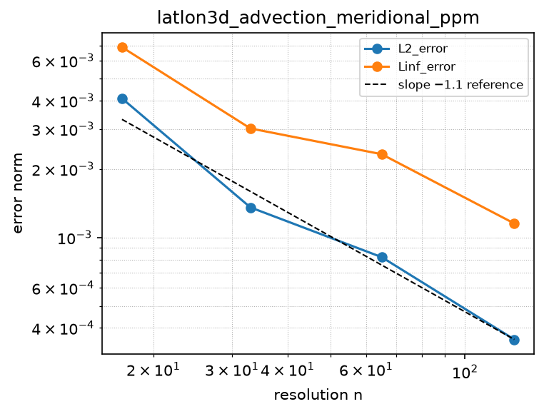
ppm_D_lev_mono_noflux_bc
Source: grids/latlon3d/rules/ppm_D_lev_mono_noflux_bc.esm
Rewrites ∂f/∂lev at priority 10 — match pattern:
{"op": "D", "args": ["f"], "wrt": "lev"}
where): fires only when f is a bare field shaped [lon, lat, lev]. Under import-edge renaming (§9.7.7) the wrt literal and this shape follow the renamed axis together, so the rule can be imported more than once (each instance scoped to its own grid) without a first-declared-wins collision. A consumer differentiating a compound inline expression must bind it to a declared shaped observed first.Discretization — one makearray tiling the output axes; boundary conditions live in the face regions of this same rule (esm-spec §9.6.8; later regions overwrite earlier, §4.3.2):
| Region | Treatment | Value |
|---|---|---|
lon ∈ [1, NLON], lat ∈ [1, NLAT], lev ∈ [4, NLEV−2] | interior | ppm_D_lev_mono_interior(f)[i,j,k] = (ppm_lev_flux_mono(f[i, j, k−2], f[i, j, k−1], f[i, j, k], f[i, j, k+1], f[i, j, k+2], dz[k−2], dz[k−1], dz[k], dz[k+1], dz[k+2], w_edge[k+1]) − ppm_lev_flux_mono(f[i, j, k−3], f[i, j, k−2], f[i, j, k−1], f[i, j, k], f[i, j, k+1], dz[k−3], dz[k−2], dz[k−1], dz[k], dz[k+1], w_edge[k])) / dz[k] for i ∈ lon, j ∈ lat, k ∈ [4, NLEV−2] |
lon ∈ [1, NLON], lat ∈ [1, NLAT], lev = 1 | boundary face | ppm_D_lev_mono_nf_k1(f)[i,j,k] = (ppm_lev_flux_mono(f[i, j, 1], f[i, j, 1], f[i, j, 1], f[i, j, 2], f[i, j, 3], dz[1], dz[1], dz[1], dz[2], dz[3], w_edge[2]) − 0) / dz[1] for i ∈ lon, j ∈ lat, k ∈ [1, 1] |
lon ∈ [1, NLON], lat ∈ [1, NLAT], lev = 2 | boundary face | ppm_D_lev_mono_nf_k2(f)[i,j,k] = (ppm_lev_flux_mono(f[i, j, 1], f[i, j, 1], f[i, j, 2], f[i, j, 3], f[i, j, 4], dz[1], dz[1], dz[2], dz[3], dz[4], w_edge[3]) − ppm_lev_flux_mono(f[i, j, 1], f[i, j, 1], f[i, j, 1], f[i, j, 2], f[i, j, 3], dz[1], dz[1], dz[1], dz[2], dz[3], w_edge[2])) / dz[2] for i ∈ lon, j ∈ lat, k ∈ [2, 2] |
lon ∈ [1, NLON], lat ∈ [1, NLAT], lev = 3 | boundary face | ppm_D_lev_mono_nf_k3(f)[i,j,k] = (ppm_lev_flux_mono(f[i, j, 1], f[i, j, 2], f[i, j, 3], f[i, j, 4], f[i, j, 5], dz[1], dz[2], dz[3], dz[4], dz[5], w_edge[4]) − ppm_lev_flux_mono(f[i, j, 1], f[i, j, 1], f[i, j, 2], f[i, j, 3], f[i, j, 4], dz[1], dz[1], dz[2], dz[3], dz[4], w_edge[3])) / dz[3] for i ∈ lon, j ∈ lat, k ∈ [3, 3] |
lon ∈ [1, NLON], lat ∈ [1, NLAT], lev = NLEV−1 | boundary face | ppm_D_lev_mono_nf_kNm1(f)[i,j,k] = (ppm_lev_flux_mono(f[i, j, NLEV−3], f[i, j, NLEV−2], f[i, j, NLEV−1], f[i, j, NLEV], f[i, j, NLEV], dz[NLEV−3], dz[NLEV−2], dz[NLEV−1], dz[NLEV], dz[NLEV], w_edge[NLEV]) − ppm_lev_flux_mono(f[i, j, NLEV−4], f[i, j, NLEV−3], f[i, j, NLEV−2], f[i, j, NLEV−1], f[i, j, NLEV], dz[NLEV−4], dz[NLEV−3], dz[NLEV−2], dz[NLEV−1], dz[NLEV], w_edge[NLEV−1])) / dz[NLEV−1] for i ∈ lon, j ∈ lat, k ∈ [NLEV−1, NLEV−1] |
lon ∈ [1, NLON], lat ∈ [1, NLAT], lev = NLEV | boundary face | ppm_D_lev_mono_nf_kN(f)[i,j,k] = (0 − ppm_lev_flux_mono(f[i, j, NLEV−3], f[i, j, NLEV−2], f[i, j, NLEV−1], f[i, j, NLEV], f[i, j, NLEV], dz[NLEV−3], dz[NLEV−2], dz[NLEV−1], dz[NLEV], dz[NLEV], w_edge[NLEV])) / dz[NLEV] for i ∈ lon, j ∈ lat, k ∈ [NLEV, NLEV] |
MONOTONE conservative flux-form vertical advection operator on the latlon3d hybrid vertical: the FULL Colella-Woodward (1984) Piecewise Parabolic Method – eq (1.6) edge interpolation built on eq (1.8) MONOTONIZED slopes, plus the eq (1.10) parabola limiter – as a finite-volume flux divergence (w u)lev with genuine no-flux top/surface boundaries, for GEOS-Chem-Classic-style vertical tracer transport. THE PRODUCTION VARIANT. Its sibling rules/ppm_D_lev_noflux_bc is the same flux-form operator with the UNLIMITED reconstruction: that one is formally 4th-order on smooth fields, but because its reconstructed edge value may overshoot the range of the two cells it separates, it introduces new extrema at a sharp vertical gradient and measurably drives a tracer NEGATIVE (verified: a boundary-layer-inversion-like step goes to -1.1e-2 under the unlimited scheme and stays bounded in [0,1] under this one). Negative concentrations are not survivable in a chemistry-transport model – they propagate into the chemistry and aerosol-thermodynamics solvers – and the usual field fix (clipping negatives to zero) silently destroys the exact mass conservation this flux form exists to provide. Vertical air-quality profiles are exactly the sharp-gradient case (capping inversion, stack plumes, surface emissions against the wall, the tropopause ozone jump), so for production tracer transport IMPORT THIS RULE; import the unlimited sibling when the field is smooth and the 4th order is wanted (it is also the accuracy ceiling this one is measured against). This matches the FV/TPCORE lineage, which selects a constrained sub-grid distribution per direction rather than the unlimited one. FLUX-FORM (like its unlimited sibling, unlike the advective-derivative horizontal ppm_D_lon/lat rules): it matches D(f, wrt: lev) but the expanded body is the conservative divergence of the vertical flux F = w*u, so a consumer writes u_t = -D(u, wrt: lev) (+ source) and the velocity enters INSIDE the operator via the free name w_edge, NOT multiplied outside. D f[i,j,k] = (F{k+1/2} - F_{k-1/2})/dz[k], with F_{k+1/2} = w_edge[k+1] * a_{k+1/2}^lim the monotone-limited upwind CW84 reconstructed tracer edge (../stencils/ppm_lev_flux_mono -> ppm_lev_edge_mono -> ppm_lev_edge_core + ppm_lev_slope_mono -> ppm_lev_slope; parabola limiter ../stencils/ppm_limit_right, reused verbatim from the zonal chain because eq (1.10) is mesh-independent). CONSERVATION IS UNAFFECTED BY LIMITING: limiting changes the reconstructed edge VALUE, never the fact that each interface has ONE flux value shared by the two cells that straddle it, so the divergence still telescopes; w_edge vanishes at the model top and surface (w_edge[1]=w_edge[NLEV+1]=0) so both wall fluxes are identically zero and total tracer mass is conserved to the bit (verified machine-zero on random data, same as the unlimited sibling). ORDER: the eq (1.8)/(1.10) limiters cannot distinguish a smooth extremum from an oscillation and clip it, so the formal order drops – measured ~2.5 (L2) / ~2.0 (Linf) on the smooth quadratic-stretch manufactured solution where the unlimited chain measures a clean 4.0. That is the deliberate trade: order you cannot realize on a real vertical profile, exchanged for boundedness you always need. The extremum-preserving Colella-Sekora (2008) limiter is the documented follow-on that would recover accuracy at genuine smooth extrema. COMPOSITIONAL BODY: a makearray tiling [lon, lat, lev] with SIX regions, each a thin apply of a factored stencil – interior cells [4, NLEV-2] use ../stencils/ppm_D_lev_mono_interior; the bottom cells k=1,2,3 use ../stencils/ppm_D_lev_mono_nf_k{1,2,3} and the top cells k=NLEV-1,NLEV use ../stencils/ppm_D_lev_mono_nf_k{Nm1,N}. FIVE boundary slabs, not the unlimited sibling’s four, because the eq (1.10) limiter needs both edges of each upwind cell and so widens the divergence support from five vertical cells to six (k-3..k+2). Requires NLEV >= 6 for a non-empty interior. Every region is a full-rank slab aggregate (output_idx [i, j, k]). FREE NAMES (consumer-supplied): dz the cell widths (grids/latlon3d lev_thickness contract, shape [lev]); w_edge the vertical velocity at cell interfaces (shape [lev_nodes], NLEV+1 values), which MUST vanish at the surface and model top for the no-flux conservation to hold (composing it with a non-vanishing w_edge is a modeling error). Match scoping: wrt: lev plus where: {f: {shape: [lon, lat, lev]}} (esm-spec 9.6.1) at priority 10 so it wins over any default-priority derivative rule sharing the lev axis. A model imports exactly ONE lev advection rule – this one or the unlimited ppm_D_lev_noflux_bc or the centered central_D_lev_zero_grad_bc, never two. Sign convention: upwind for w >= 0 (upward); a sign-general variant belongs in a separate rule. NOTE: the horizontal ppm_D_lon/ppm_D_lat rules currently limit with eq (1.10) only (their ppm_face_value edge uses unlimited slopes, i.e. no eq (1.8)), so they are not as tightly bounded as this vertical chain; upgrading them to the full monotone reconstruction is a documented follow-on. Bit-faithful TPCORE (Courant-integral semi-Lagrangian) and true Psurf-coupled 3-D dp[i,j,k] remain follow-ons (grids/latlon3d/grid.esm).
References
- Colella, P., & Woodward, P. R. (1984). The Piecewise Parabolic Method (PPM) for gas-dynamical simulations. Journal of Computational Physics, 54(1), 174-201.
doi:10.1016/0021-9991(84)90143-8 - Lin, S.-J., & Rood, R. B. (1996). Multidimensional flux-form semi-Lagrangian transport schemes. Monthly Weather Review, 124(9), 2046-2070. Flux-form finite-volume vertical transport (the GEOS-Chem/TPCORE lineage; production TPCORE selects a constrained/positive-definite sub-grid distribution per direction rather than the unlimited one).
doi:10.1175/1520-0493(1996)124<2046:MFFSLT>2.0.CO;2 - Colella, P., & Sekora, M. D. (2008). A limiter for PPM that preserves accuracy at smooth extrema. Journal of Computational Physics, 227(15), 7069-7076. The documented follow-on that would recover high order at genuine smooth extrema.
doi:10.1016/j.jcp.2008.03.034
Conformance fixtures
- ast:
latlon3d_ppm_D_lev_mono_noflux_bc— statusactive - convergence:
latlon3d_advection_vertical_ppm_mono— statusactive
Convergence — case latlon3d_advection_vertical_ppm_mono
Error norms read from the committed golden tests/conformance/convergence/latlon3d_advection_vertical_ppm_mono/golden/errors.json (binding: julia; nothing recomputed for display).
| n | L2_error | observed order | Linf_error | observed order |
|---|---|---|---|---|
| 8 | 5.647e-03 | — | 7.081e-03 | — |
| 16 | 1.134e-03 | 2.32 | 2.179e-03 | 1.70 |
| 32 | 2.095e-04 | 2.44 | 5.742e-04 | 1.92 |
| 64 | 3.764e-05 | 2.48 | 1.462e-04 | 1.97 |
Expected order: 2.2 (± 0.4).
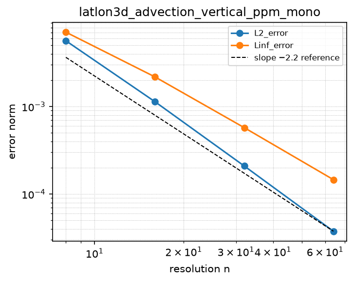
ppm_D_lev_noflux_bc
Source: grids/latlon3d/rules/ppm_D_lev_noflux_bc.esm
Rewrites ∂f/∂lev at priority 10 — match pattern:
{"op": "D", "args": ["f"], "wrt": "lev"}
where): fires only when f is a bare field shaped [lon, lat, lev]. Under import-edge renaming (§9.7.7) the wrt literal and this shape follow the renamed axis together, so the rule can be imported more than once (each instance scoped to its own grid) without a first-declared-wins collision. A consumer differentiating a compound inline expression must bind it to a declared shaped observed first.Discretization — one makearray tiling the output axes; boundary conditions live in the face regions of this same rule (esm-spec §9.6.8; later regions overwrite earlier, §4.3.2):
| Region | Treatment | Value |
|---|---|---|
lon ∈ [1, NLON], lat ∈ [1, NLAT], lev ∈ [3, NLEV−2] | interior | ppm_D_lev_interior(f)[i,j,k] = (ppm_lev_flux(f[i, j, k−1], f[i, j, k], f[i, j, k+1], f[i, j, k+2], dz[k−1], dz[k], dz[k+1], dz[k+2], w_edge[k+1]) − ppm_lev_flux(f[i, j, k−2], f[i, j, k−1], f[i, j, k], f[i, j, k+1], dz[k−2], dz[k−1], dz[k], dz[k+1], w_edge[k])) / dz[k] for i ∈ lon, j ∈ lat, k ∈ [3, NLEV−2] |
lon ∈ [1, NLON], lat ∈ [1, NLAT], lev = 1 | boundary face | ppm_D_lev_nf_k1(f)[i,j,k] = (ppm_lev_flux(f[i, j, 1], f[i, j, 1], f[i, j, 2], f[i, j, 3], dz[1], dz[1], dz[2], dz[3], w_edge[2]) − 0) / dz[1] for i ∈ lon, j ∈ lat, k ∈ [1, 1] |
lon ∈ [1, NLON], lat ∈ [1, NLAT], lev = 2 | boundary face | ppm_D_lev_nf_k2(f)[i,j,k] = (ppm_lev_flux(f[i, j, 1], f[i, j, 2], f[i, j, 3], f[i, j, 4], dz[1], dz[2], dz[3], dz[4], w_edge[3]) − ppm_lev_flux(f[i, j, 1], f[i, j, 1], f[i, j, 2], f[i, j, 3], dz[1], dz[1], dz[2], dz[3], w_edge[2])) / dz[2] for i ∈ lon, j ∈ lat, k ∈ [2, 2] |
lon ∈ [1, NLON], lat ∈ [1, NLAT], lev = NLEV−1 | boundary face | ppm_D_lev_nf_kNm1(f)[i,j,k] = (ppm_lev_flux(f[i, j, NLEV−2], f[i, j, NLEV−1], f[i, j, NLEV], f[i, j, NLEV], dz[NLEV−2], dz[NLEV−1], dz[NLEV], dz[NLEV], w_edge[NLEV]) − ppm_lev_flux(f[i, j, NLEV−3], f[i, j, NLEV−2], f[i, j, NLEV−1], f[i, j, NLEV], dz[NLEV−3], dz[NLEV−2], dz[NLEV−1], dz[NLEV], w_edge[NLEV−1])) / dz[NLEV−1] for i ∈ lon, j ∈ lat, k ∈ [NLEV−1, NLEV−1] |
lon ∈ [1, NLON], lat ∈ [1, NLAT], lev = NLEV | boundary face | ppm_D_lev_nf_kN(f)[i,j,k] = (0 − ppm_lev_flux(f[i, j, NLEV−2], f[i, j, NLEV−1], f[i, j, NLEV], f[i, j, NLEV], dz[NLEV−2], dz[NLEV−1], dz[NLEV], dz[NLEV], w_edge[NLEV])) / dz[NLEV] for i ∈ lon, j ∈ lat, k ∈ [NLEV, NLEV] |
Conservative flux-form vertical advection operator on the latlon3d hybrid vertical: the Piecewise Parabolic Method (Colella & Woodward 1984) finite-volume flux divergence (w u)lev with genuine no-flux top/surface boundaries, for GEOS-Chem-Classic-style vertical tracer transport. Unlike the advective-derivative sibling central_D_lev_zero_grad_bc (and the horizontal ppm_D_lon/lat rules, which discretize the plain derivative), THIS rule is FLUX-FORM: it matches D(f, wrt: lev) but the expanded body is the conservative divergence of the vertical flux F = w*u, so a consumer writes u_t = -D(u, wrt: lev) (+ source) and gets exactly mass-conserving vertical advection – the velocity enters INSIDE the operator via the free name w_edge, and is NOT multiplied outside. D f[i,j,k] = (F{k+1/2} - F_{k-1/2})/dz[k], with F_{k+1/2} = w_edge[k+1] * a_{k+1/2} the upwind CW84 non-uniform 4th-order reconstructed tracer edge (../stencils/ppm_lev_flux -> ppm_lev_edge -> ppm_lev_slope) scaled by the interface velocity. NO-FLUX / CONSERVATION: the vertical velocity w_edge vanishes at the model top and surface (w_edge[1]=w_edge[NLEV+1]=0), so both wall fluxes are identically zero and, because every interior interface flux is written byte-identically in the two cells that share it, sum over k of (D f * dz) telescopes to (top flux - surface flux) = 0 – total tracer mass is conserved to the bit (a genuine finite-volume no-flux closure, not a forced zero-gradient one; this is why the vertical PPM is flux-form while lon/lat are advective-derivative form). ORDER: verified 4th-order in both L2 and Linf with exact conservation on the quadratic-stretch mesh (UNLIMITED reconstruction). NOT MONOTONE – the monotone variant IS NOW SHIPPED as the sibling rules/ppm_D_lev_mono_noflux_bc (full CW84: eq (1.6) edge on eq (1.8) monotonized slopes, plus the eq (1.10) parabola limiter), which is the PRODUCTION choice – this unlimited chain is measurably NOT bounded (a boundary-layer-inversion-like step drives the tracer to -1.1e-2, and adversarial profiles go further negative), so use it only where the field is smooth and the 4th order is wanted; it remains the accuracy ceiling the monotone rule is measured against. The monotone sibling measures ~2.4 (L2) / ~1.9 (Linf); that gap IS the price of boundedness. WELL-POSEDNESS: the forced-steady manufactured-solution test integrates as a finite-time initial-value problem (the operator’s constant null mode – w vanishing at both walls – drifts only marginally over the short assert window, exactly as the other advection convergence cases integrate), so the observed 4th-order drift is clean. COMPOSITIONAL BODY: a makearray tiling [lon, lat, lev] with five regions, each a thin apply of a factored stencil – interior cells [3, NLEV-2] use ../stencils/ppm_D_lev_interior; the bottom cells k=1,2 use ../stencils/ppm_D_lev_nf_k{1,2} and the top cells k=NLEV-1,NLEV use ../stencils/ppm_D_lev_nf_k{Nm1,N} (the 5-cell support needs two ghost-filled cells at each wall, with zero-gradient sub-surface/above-top ghosts and the zero wall flux). Every region is a full-rank slab aggregate (output_idx [i, j, k]). FREE NAMES (consumer-supplied): dz the cell widths (grids/latlon3d lev_thickness contract, shape [lev]); w_edge the vertical velocity at cell interfaces (shape [lev_nodes], NLEV+1 values), which MUST vanish at the surface and model top for the no-flux conservation to hold (composing it with a non-vanishing w_edge is a modeling error). Match scoping: wrt: lev plus where: {f: {shape: [lon, lat, lev]}} (esm-spec 9.6.1) at priority 10 so it wins over any default-priority derivative rule sharing the lev axis and fires only on the vertical operator of a bare field over THIS grid’s lon x lat x lev index sets; under import-edge renaming (esm-spec 9.7.7) the wrt literal and the where shape follow together. A model imports exactly one lev advection rule. Sign convention: upwind for w >= 0 (upward); a sign-general variant belongs in a separate rule. Bit-faithful TPCORE (Courant-integral semi-Lagrangian) and true Psurf-coupled 3-D dp[i,j,k] remain documented follow-ons (grids/latlon3d/grid.esm).
References
- Colella, P., & Woodward, P. R. (1984). The Piecewise Parabolic Method (PPM) for gas-dynamical simulations. Journal of Computational Physics, 54(1), 174-201.
doi:10.1016/0021-9991(84)90143-8 - Lin, S.-J., & Rood, R. B. (1996). Multidimensional flux-form semi-Lagrangian transport schemes. Monthly Weather Review, 124(9), 2046-2070. Flux-form finite-volume vertical transport (the GEOS-Chem/TPCORE lineage).
doi:10.1175/1520-0493(1996)124<2046:MFFSLT>2.0.CO;2
Conformance fixtures
- ast:
latlon3d_ppm_D_lev_noflux_bc— statusactive - convergence:
latlon3d_advection_vertical_ppm— statusactive
Convergence — case latlon3d_advection_vertical_ppm
Error norms read from the committed golden tests/conformance/convergence/latlon3d_advection_vertical_ppm/golden/errors.json (binding: julia; nothing recomputed for display).
| n | L2_error | observed order | Linf_error | observed order |
|---|---|---|---|---|
| 16 | 2.644e-05 | — | 5.400e-05 | — |
| 32 | 1.689e-06 | 3.97 | 3.928e-06 | 3.78 |
| 64 | 1.061e-07 | 3.99 | 2.609e-07 | 3.91 |
| 128 | 6.639e-09 | 4.00 | 1.675e-08 | 3.96 |
Expected order: 4 (± 0.3).
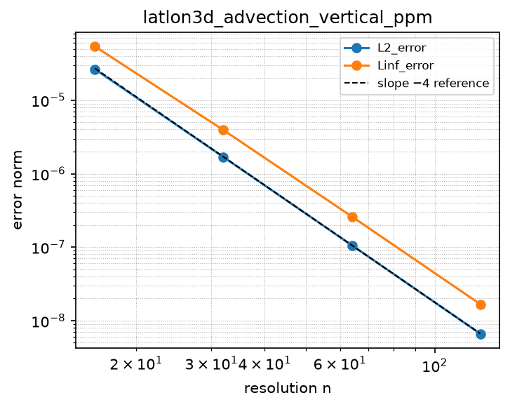
ppm_D_lon_periodic
Source: grids/latlon3d/rules/ppm_D_lon_periodic.esm
Rewrites ∂f/∂lon at priority 10 — match pattern:
{"op": "D", "args": ["f"], "wrt": "lon"}
where): fires only when f is a bare field shaped [lon, lat, lev]. Under import-edge renaming (§9.7.7) the wrt literal and this shape follow the renamed axis together, so the rule can be imported more than once (each instance scoped to its own grid) without a first-declared-wins collision. A consumer differentiating a compound inline expression must bind it to a declared shaped observed first.Discretization — one makearray tiling the output axes; boundary conditions live in the face regions of this same rule (esm-spec §9.6.8; later regions overwrite earlier, §4.3.2):
| Region | Treatment | Value |
|---|---|---|
lon ∈ [4, NLON−2], lat ∈ [1, NLAT], lev ∈ [1, NLEV] | interior | ppm_D_lon_interior(f)[i,j,k] = (ppm_flux(f[i−2, j, k], f[i−1, j, k], f[i, j, k], f[i+1, j, k], f[i+2, j, k]) − ppm_flux(f[i−3, j, k], f[i−2, j, k], f[i−1, j, k], f[i, j, k], f[i+1, j, k])) / dlon_deg for i ∈ [4, NLON−2], j ∈ lat, k ∈ lev |
lon = 1, lat ∈ [1, NLAT], lev ∈ [1, NLEV] | boundary face | ppm_D_lon_wrap_col1(f)[i,j,k] = (ppm_flux(f[NLON−1, j, k], f[NLON, j, k], f[1, j, k], f[2, j, k], f[3, j, k]) − ppm_flux(f[NLON−2, j, k], f[NLON−1, j, k], f[NLON, j, k], f[1, j, k], f[2, j, k])) / dlon_deg for i ∈ [1, 1], j ∈ lat, k ∈ lev |
lon = 2, lat ∈ [1, NLAT], lev ∈ [1, NLEV] | boundary face | ppm_D_lon_wrap_col2(f)[i,j,k] = (ppm_flux(f[NLON, j, k], f[1, j, k], f[2, j, k], f[3, j, k], f[4, j, k]) − ppm_flux(f[NLON−1, j, k], f[NLON, j, k], f[1, j, k], f[2, j, k], f[3, j, k])) / dlon_deg for i ∈ [2, 2], j ∈ lat, k ∈ lev |
lon = 3, lat ∈ [1, NLAT], lev ∈ [1, NLEV] | boundary face | ppm_D_lon_wrap_col3(f)[i,j,k] = (ppm_flux(f[1, j, k], f[2, j, k], f[3, j, k], f[4, j, k], f[5, j, k]) − ppm_flux(f[NLON, j, k], f[1, j, k], f[2, j, k], f[3, j, k], f[4, j, k])) / dlon_deg for i ∈ [3, 3], j ∈ lat, k ∈ lev |
lon = NLON−1, lat ∈ [1, NLAT], lev ∈ [1, NLEV] | boundary face | ppm_D_lon_wrap_colNm1(f)[i,j,k] = (ppm_flux(f[NLON−3, j, k], f[NLON−2, j, k], f[NLON−1, j, k], f[NLON, j, k], f[1, j, k]) − ppm_flux(f[NLON−4, j, k], f[NLON−3, j, k], f[NLON−2, j, k], f[NLON−1, j, k], f[NLON, j, k])) / dlon_deg for i ∈ [NLON−1, NLON−1], j ∈ lat, k ∈ lev |
lon = NLON, lat ∈ [1, NLAT], lev ∈ [1, NLEV] | boundary face | ppm_D_lon_wrap_colN(f)[i,j,k] = (ppm_flux(f[NLON−2, j, k], f[NLON−1, j, k], f[NLON, j, k], f[1, j, k], f[2, j, k]) − ppm_flux(f[NLON−3, j, k], f[NLON−2, j, k], f[NLON−1, j, k], f[NLON, j, k], f[1, j, k])) / dlon_deg for i ∈ [NLON, NLON], j ∈ lat, k ∈ lev |
Piecewise Parabolic Method (PPM; Colella & Woodward 1984) conservative finite-volume zonal first derivative u_lon on the latlon3d grid with a periodic (wrap) longitude boundary, for zonal advection with non-negative angular velocity (a consumer writes u_t = -omega_deg*D(u, wrt: lon), omega_deg >= 0) in a 3-D tracer-transport model such as GEOS-Chem Classic. The rank-3 (lon x lat x lev) extension of grids/cartesian_uniform_1d/rules/ppm_D_periodic, applied on every (lat, lev) column; a higher-order GC-faithful alternative to the sibling first-order upwind1_D_lon_periodic. Matches D(f, wrt: lon), a PER-DEGREE derivative. FLUX FORM: the SEMI-DISCRETE (method-of-lines) reconstructed-edge flux F_{i+1/2} = qr_lim(cell i), the CW84-limited right-edge value of the upwind (west) cell – NOT the fully-discrete Courant-integral flux. The Courant form needs the CFL number inside the operator; the ESS simulate() pathway is method-of-lines (the rule supplies only the spatial operator D(u,lon) and the ODE integrator owns dt, exactly like the sibling upwind1_D_lon_periodic / central_D_lon rules), so the semi-discrete edge-value flux is the composable choice, faithful to GC’s PPM reconstruction but not its TPCORE Courant integral (see grids/latlon3d/grid.esm for the deferred bit-faithful TPCORE note). D f[i,j,k] = (F_{i+1/2} - F_{i-1/2})/dlon_deg; because adjacent zonal cells share the identical float face flux the divergence telescopes and the periodic ring conserves sum(f) to the bit. COMPOSITIONAL BODY: a makearray tiling [lon, lat, lev] with exactly six regions, each filled by a thin apply of a factored stencil – interior columns [4, NLON-2] x lat x lev use ../stencils/ppm_D_lon_interior; the low wrap columns i=1,2,3 and high wrap columns i=NLON-1,NLON use the five ../stencils/ppm_D_lon_wrap_col{1,2,3,Nm1,N} slab faces (PPM’s 5-cell support needs three wrap columns at the low end and two at the high end). Every region is a full-rank slab aggregate (output_idx [i, j, k]) so every binding’s simulator fills the wrap slabs without rank promotion. RECONSTRUCTION: raw edges are CW84 eq.(1.6) 4th-order interpolation; the unlimited flux-difference reduces exactly to the 4th-order central first derivative, so away from extrema the scheme is high order. LIMITER: CW84 eqs.(1.7)-(1.10) monotonicity limiter (stencils/ppm_limit_right). ORDER (honest, observed): on a smooth zonal MMS the CW84 limiter still activates at the smooth extrema of the m=1 wave (the classic clipping of the original 1984 limiter, cured only by later extremum-preserving variants), flattening the parabola there, so the global convergence is sub-nominal and norm-dependent – see tests/conformance/convergence/latlon3d_advection_zonal_ppm for the observed order. MONOTONICITY: with the eq. (1.8) + eq. (1.10) reconstruction the semi-discrete form is bounded in practice (a non-negative field with sharp jumps stays exactly within its initial range in the in-pipeline tests above) but it is still NOT a proven TVD/positivity theorem – a strict guarantee would require the fully-discrete Courant-integral form under a CFL condition, which the method-of-lines pathway cannot carry. Match scoping: wrt: lon plus where: {f: {shape: [lon, lat, lev]}} (esm-spec 9.6.1) at priority 10 (mirroring the cartesian ppm sibling) so it wins over any default-priority first-derivative rule sharing the lon axis and fires only on the longitudinal derivative of a bare field declared over THIS grid’s lon x lat x lev index sets; under import-edge renaming (esm-spec 9.7.7) the wrt literal and the where shape follow the renamed axis together, so two latlon3d instances coexist. The constraint requires a bare shaped field; a consumer differentiating a compound expression must bind it to a declared lon x lat x lev observed first. dlon_deg is the inherited consumer-supplied zonal spacing free name (grids/latlon3d/grid.esm); the periodic wrap is dlon_deg-scale-invariant. Sign convention: upwind for flow toward +lon; a westward variant belongs in a separate rule. *** MONOTONICITY UPGRADE (2026-07-13) – READ THIS. *** This rule is now genuinely BOUNDED. Its flux (../stencils/ppm_flux) previously reconstructed edges with the UNLIMITED eq. (1.7) slopes and relied on the eq. (1.10) parabola limiter alone; that combination does NOT bound the scheme. Verified in-pipeline on rules/ppm_D_periodic with sharp non-negative initial data (square / spike / sawtooth at N=32/64/128): the old chain drove a tracer in [0,1] down to -5.3e-2 and up to 1.053, i.e. it manufactured negative concentrations – not survivable in a chemistry-transport model, where they propagate into the chemistry and aerosol solvers, and where the usual fix (clip to zero) silently destroys mass conservation. The edges are now built on the CW84 eq. (1.8) MONOTONIZED slopes (../stencils/ppm_face_value_mono -> ppm_slope_mono), and the same in-pipeline test now holds the tracer EXACTLY in [0, 1] (min 0.0, max 1.0) on every profile and resolution. BOTH limiters are load-bearing and neither alone suffices: eq. (1.8) forces the interpolated EDGE to lie between the two cells it separates, while eq. (1.10)’s extremum-flattening branch is what stops outflux from a local minimum. (Independently re-derived on the stretched vertical; see grids/latlon3d/rules/ppm_D_lev_mono_noflux_bc.) ORDER CONSEQUENCES (honest): on a smooth MMS the upgrade IMPROVES the observed order for the periodic cases (1-D 1.5 -> 1.87 L2; zonal 1.64 -> 1.88 L2), because eq.(1.10)-alone clips more erratically. But where the manufactured solution has a SMOOTH INTERIOR EXTREMUM the upgrade LOWERS it: the meridional cos^4 case falls from 2.00 to 1.22 (L2), because eq. (1.8) zeroes the slope at the extremum cell and that zero also pollutes the two neighbouring edges. That is the classic 1984-limiter smooth-extremum clip, and it is the price of boundedness; the extremum-preserving Colella-Sekora (2008) limiter is the documented follow-on that would recover the order while keeping the bound. COST: the lowered AST grows ~8.5x, because ppm_limit_right must inline both edges ~5x each and a let-free AST cannot share them, so the now-larger monotonized edge is paid for ten times over; a CSE/let construct in ESM would remove this (documented follow-on). The rule’s regions, stencil support (5 cells) and boundary faces are UNCHANGED – only the edge reconstruction inside ppm_flux changed – so this is a drop-in fix, not a new operator.
References
- Colella, P., & Woodward, P. R. (1984). The Piecewise Parabolic Method (PPM) for gas-dynamical simulations. Journal of Computational Physics, 54(1), 174-201.
doi:10.1016/0021-9991(84)90143-8 - Lin, S.-J., & Rood, R. B. (1996). Multidimensional flux-form semi-Lagrangian transport schemes. Monthly Weather Review, 124(9), 2046-2070. Flux-form finite-volume advection composition (the GEOS-Chem/TPCORE lineage).
doi:10.1175/1520-0493(1996)124<2046:MFFSLT>2.0.CO;2 - Colella, P., & Sekora, M. D. (2008). A limiter for PPM that preserves accuracy at smooth extrema. Journal of Computational Physics, 227(15), 7069-7076.
doi:10.1016/j.jcp.2008.03.034
Conformance fixtures
- ast:
latlon3d_ppm_D_lon_periodic— statusactive - convergence:
latlon3d_advection_zonal_ppm— statusactive
Convergence — case latlon3d_advection_zonal_ppm
Error norms read from the committed golden tests/conformance/convergence/latlon3d_advection_zonal_ppm/golden/errors.json (binding: julia; nothing recomputed for display).
| n | L2_error | observed order | Linf_error | observed order |
|---|---|---|---|---|
| 16 | 3.173e-02 | — | 4.229e-02 | — |
| 32 | 9.021e-03 | 1.81 | 1.446e-02 | 1.55 |
| 64 | 2.447e-03 | 1.88 | 3.787e-03 | 1.93 |
| 128 | 6.484e-04 | 1.92 | 1.819e-03 | 1.06 |
Expected order: 1.7 (± 0.3).
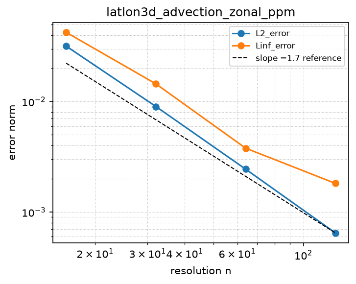
ppm_flux_D_lat_mono_inflow_bc
Source: grids/latlon3d/rules/ppm_flux_D_lat_mono_inflow_bc.esm
Rewrites D(V·q, qbc_s, qbc_n) at priority 10 — match pattern:
{"op": "D", "args": [{"op": "*", "args": ["V", "q"]}, "qbc_s", "qbc_n"], "wrt": "lat"}
where): fires only when V is a bare field shaped [lon, lat_nodes, lev]. Under import-edge renaming (§9.7.7) the wrt literal and this shape follow the renamed axis together, so the rule can be imported more than once (each instance scoped to its own grid) without a first-declared-wins collision. A consumer differentiating a compound inline expression must bind it to a declared shaped observed first.Discretization — one makearray tiling the output axes; boundary conditions live in the face regions of this same rule (esm-spec §9.6.8; later regions overwrite earlier, §4.3.2):
| Region | Treatment | Value |
|---|---|---|
lon ∈ [1, NLON], lat ∈ [4, NLAT−3], lev ∈ [1, NLEV] | interior | ppmflux_D_lat_interior(q, V)[i,j,k] = (ppmflux_lev_face_flux(q[i, j−2, k], q[i, j−1, k], q[i, j, k], q[i, j+1, k], q[i, j+2, k], q[i, j+3, k], dphi_lat[j−2], dphi_lat[j−1], dphi_lat[j], dphi_lat[j+1], dphi_lat[j+2], dphi_lat[j+3], V[i, j+1, k])·coslat_e[j+1] − ppmflux_lev_face_flux(q[i, j−3, k], q[i, j−2, k], q[i, j−1, k], q[i, j, k], q[i, j+1, k], q[i, j+2, k], dphi_lat[j−3], dphi_lat[j−2], dphi_lat[j−1], dphi_lat[j], dphi_lat[j+1], dphi_lat[j+2], V[i, j, k])·coslat_e[j]) / dS_lat[j] for i ∈ lon, j ∈ [4, NLAT−3], k ∈ lev |
lon ∈ [1, NLON], lat = 1, lev ∈ [1, NLEV] | boundary face | ppmflux_D_lat_inflow_j1(q, V, qbc_s)[i,j,k] = (ppmflux_lev_face_flux(qbc_s[i, k], qbc_s[i, k], q[i, 1, k], q[i, 2, k], q[i, 3, k], q[i, 4, k], dphi_lat[1], dphi_lat[1], dphi_lat[1], dphi_lat[2], dphi_lat[3], dphi_lat[4], V[i, 2, k])·coslat_e[2] − ppmflux_lev_face_flux(qbc_s[i, k], qbc_s[i, k], qbc_s[i, k], q[i, 1, k], q[i, 2, k], q[i, 3, k], dphi_lat[1], dphi_lat[1], dphi_lat[1], dphi_lat[1], dphi_lat[2], dphi_lat[3], V[i, 1, k])·coslat_e[1]) / dS_lat[1] for i ∈ lon, j ∈ [1, 1], k ∈ lev |
lon ∈ [1, NLON], lat = 2, lev ∈ [1, NLEV] | boundary face | ppmflux_D_lat_inflow_j2(q, V, qbc_s)[i,j,k] = (ppmflux_lev_face_flux(qbc_s[i, k], q[i, 1, k], q[i, 2, k], q[i, 3, k], q[i, 4, k], q[i, 5, k], dphi_lat[1], dphi_lat[1], dphi_lat[2], dphi_lat[3], dphi_lat[4], dphi_lat[5], V[i, 3, k])·coslat_e[3] − ppmflux_lev_face_flux(qbc_s[i, k], qbc_s[i, k], q[i, 1, k], q[i, 2, k], q[i, 3, k], q[i, 4, k], dphi_lat[1], dphi_lat[1], dphi_lat[1], dphi_lat[2], dphi_lat[3], dphi_lat[4], V[i, 2, k])·coslat_e[2]) / dS_lat[2] for i ∈ lon, j ∈ [2, 2], k ∈ lev |
lon ∈ [1, NLON], lat = 3, lev ∈ [1, NLEV] | boundary face | ppmflux_D_lat_inflow_j3(q, V, qbc_s)[i,j,k] = (ppmflux_lev_face_flux(q[i, 1, k], q[i, 2, k], q[i, 3, k], q[i, 4, k], q[i, 5, k], q[i, 6, k], dphi_lat[1], dphi_lat[2], dphi_lat[3], dphi_lat[4], dphi_lat[5], dphi_lat[6], V[i, 4, k])·coslat_e[4] − ppmflux_lev_face_flux(qbc_s[i, k], q[i, 1, k], q[i, 2, k], q[i, 3, k], q[i, 4, k], q[i, 5, k], dphi_lat[1], dphi_lat[1], dphi_lat[2], dphi_lat[3], dphi_lat[4], dphi_lat[5], V[i, 3, k])·coslat_e[3]) / dS_lat[3] for i ∈ lon, j ∈ [3, 3], k ∈ lev |
lon ∈ [1, NLON], lat = NLAT−2, lev ∈ [1, NLEV] | boundary face | ppmflux_D_lat_inflow_jNm2(q, V, qbc_n)[i,j,k] = (ppmflux_lev_face_flux(q[i, NLAT−4, k], q[i, NLAT−3, k], q[i, NLAT−2, k], q[i, NLAT−1, k], q[i, NLAT, k], qbc_n[i, k], dphi_lat[NLAT−4], dphi_lat[NLAT−3], dphi_lat[NLAT−2], dphi_lat[NLAT−1], dphi_lat[NLAT], dphi_lat[NLAT], V[i, NLAT−1, k])·coslat_e[NLAT−1] − ppmflux_lev_face_flux(q[i, NLAT−5, k], q[i, NLAT−4, k], q[i, NLAT−3, k], q[i, NLAT−2, k], q[i, NLAT−1, k], q[i, NLAT, k], dphi_lat[NLAT−5], dphi_lat[NLAT−4], dphi_lat[NLAT−3], dphi_lat[NLAT−2], dphi_lat[NLAT−1], dphi_lat[NLAT], V[i, NLAT−2, k])·coslat_e[NLAT−2]) / dS_lat[NLAT−2] for i ∈ lon, j ∈ [NLAT−2, NLAT−2], k ∈ lev |
lon ∈ [1, NLON], lat = NLAT−1, lev ∈ [1, NLEV] | boundary face | ppmflux_D_lat_inflow_jNm1(q, V, qbc_n)[i,j,k] = (ppmflux_lev_face_flux(q[i, NLAT−3, k], q[i, NLAT−2, k], q[i, NLAT−1, k], q[i, NLAT, k], qbc_n[i, k], qbc_n[i, k], dphi_lat[NLAT−3], dphi_lat[NLAT−2], dphi_lat[NLAT−1], dphi_lat[NLAT], dphi_lat[NLAT], dphi_lat[NLAT], V[i, NLAT, k])·coslat_e[NLAT] − ppmflux_lev_face_flux(q[i, NLAT−4, k], q[i, NLAT−3, k], q[i, NLAT−2, k], q[i, NLAT−1, k], q[i, NLAT, k], qbc_n[i, k], dphi_lat[NLAT−4], dphi_lat[NLAT−3], dphi_lat[NLAT−2], dphi_lat[NLAT−1], dphi_lat[NLAT], dphi_lat[NLAT], V[i, NLAT−1, k])·coslat_e[NLAT−1]) / dS_lat[NLAT−1] for i ∈ lon, j ∈ [NLAT−1, NLAT−1], k ∈ lev |
lon ∈ [1, NLON], lat = NLAT, lev ∈ [1, NLEV] | boundary face | ppmflux_D_lat_inflow_jN(q, V, qbc_n)[i,j,k] = (ppmflux_lev_face_flux(q[i, NLAT−2, k], q[i, NLAT−1, k], q[i, NLAT, k], qbc_n[i, k], qbc_n[i, k], qbc_n[i, k], dphi_lat[NLAT−2], dphi_lat[NLAT−1], dphi_lat[NLAT], dphi_lat[NLAT], dphi_lat[NLAT], dphi_lat[NLAT], V[i, NLAT+1, k])·coslat_e[NLAT+1] − ppmflux_lev_face_flux(q[i, NLAT−3, k], q[i, NLAT−2, k], q[i, NLAT−1, k], q[i, NLAT, k], qbc_n[i, k], qbc_n[i, k], dphi_lat[NLAT−3], dphi_lat[NLAT−2], dphi_lat[NLAT−1], dphi_lat[NLAT], dphi_lat[NLAT], dphi_lat[NLAT], V[i, NLAT, k])·coslat_e[NLAT]) / dS_lat[NLAT] for i ∈ lon, j ∈ [NLAT, NLAT], k ∈ lev |
UPWIND-BIASED, MONOTONE, conservative flux-form MERIDIONAL advection D(Vq, wrt: lat) on the latlon3d grid for a REGIONAL (limited-area) domain with OPEN lateral boundaries: a prescribed lateral-boundary concentration (Dirichlet inflow) carried in through whichever wall the wind blows INTO, and the interior reconstruction carried out through whichever wall it blows OUT of. The open-boundary sibling of rules/ppm_flux_D_lat_mono_polar: identical interior, identical spherical metric, identical CW84 eq (1.6)/(1.8)/(1.10) limited reconstruction and sign-of-velocity donor selection (../stencils/ppmflux_lev_face_flux), and the SAME seven-cell support – only the boundary closure differs. The periodic rule ROTATES the ghost indices around the sphere and the polar rule OMITS the pole-wall flux; this rule FORMS each open wall flux from a prescribed exterior halo instead. THE HALO IS THE BOUNDARY RECONSTRUCTION (full order, not donor). Near each wall the seven-cell reconstruction reaches for out-of-domain cells; those are supplied by the boundary concentrations qbc_s (south, shape [lon, lev]) and qbc_n (north), a constant halo along the wall at each level, passed as OPERANDS of the matched derivative. The wall face flux is then the CW84-limited one-sided reconstruction over that halo, upwind-selected: F = max(w,0)aR_ext + min(w,0)aL_int, so on INFLOW (w into the domain) the prescribed halo is donated and on OUTFLOW the interior parabola leaves. Each of the two walls handles BOTH regimes by the sign of the wall-normal wind – strictly more general than the 1-D grids/cartesian_uniform_1d/rules/ppm_D_inflow_bc, which hard-codes one inflow wall and one outflow wall for a one-signed speed. CONSISTENCY WITH CONTINUITY / FREE-STREAM. At q == 1 with the halo == 1, every CW84 correction term is a difference of equal values and is exactly 0.0 in IEEE, each parabola is the constant 1, every wall flux collapses to F = w exactly, and the tendency is BITWISE the pure mass divergence: a tracer carried as mq alongside the air mass m stays exactly equal through the open walls (gated by tests/conformance/simulation/latlon3d_transport_cwc_regional_inflow). CONSERVATION. Every INTERIOR interface face is built from the SAME atom, cells, widths and face velocity in the two cells that share it (the boundary slabs are ../stencils/ppmflux_D_lat_interior with only the out-of-domain gathers rerouted to the halo), so the flux divergence telescopes to the bit; the domain is OPEN, so the column/row integral is NOT invariant – mass enters and leaves through the wall fluxes, which is the point. On OUTFLOW the boundary-cell reconstruction is mildly influenced by the halo (as in operational regional CTM lateral-boundary schemes); a per-wall non-reflecting extrapolation outflow is a documented follow-on. It never breaks conservation (the wall face is single-valued). COMPOUND MATCH. D(Vq, qbc_s, qbc_n, wrt: lat) at priority 10 with the wind on the LEFT of the product and a where-shape constraint separating the face-staggered wind (V over [’lon’, ’lat_nodes’, ’lev’]) from the cell tracer q – the same contract as the periodic/polar siblings. Carrying the halo as operands also makes this rule’s match STRUCTURALLY distinct from its periodic/polar siblings — 3 operands against their 1 — so it no longer collides with them at priority 10 and a problem may import it ALONGSIDE a periodic/polar rule for the same axis: the arity of each call site selects the scheme. (Its where guard on the face-staggered wind is still what separates it from the same-priority face_flux_divergence_lat_open_bc, which also matches a product under D.) PER-TRACER HALO. qbc_s and qbc_n are rule PARAMS, bound by the match from the lat derivative’s 2nd and 3rd operands — not free names read out of the consumer’s scope. This is what lets each advected tracer carry its OWN lateral boundary concentration: a chemical mechanism advecting 12 species writes D(MxO3, O3_bc_w, O3_bc_e, wrt: lat) beside D(MxNO, NO_bc_w, NO_bc_e, wrt: lat), and the two halos are independent. (Were they free names, every tracer lowered against this rule would necessarily SHARE one boundary field — there would be no way to give O3 a 40 ppb inflow and NO a 0.0004 ppb one.) It is the same contract EarthSciAST’s own grad(f, inflow) inflow fixture uses. The geometry names (dphi_lat, dS_lat, …) ARE still read from the consumer’s scope, the same contract by which the vertical flux stencils read dz. Semi-discrete (method-of-lines): the ODE integrator owns dt. Requires NLAT >= 7 for a non-empty interior.
References
- Colella, P., & Woodward, P. R. (1984). The Piecewise Parabolic Method (PPM) for gas-dynamical simulations. Journal of Computational Physics, 54(1), 174-201.
doi:10.1016/0021-9991(84)90143-8 - Lin, S.-J., & Rood, R. B. (1996). Multidimensional flux-form semi-Lagrangian transport schemes. Monthly Weather Review, 124(9), 2046-2070.
doi:10.1175/1520-0493(1996)124<2046:MFFSLT>2.0.CO;2 - LeVeque, R. J. (2002). Finite Volume Methods for Hyperbolic Problems. Cambridge University Press. Section 7 (inflow / outflow boundary conditions for advection) and Section 4.1 (the upwind donor flux).
- Colella, P., & Sekora, M. D. (2008). A limiter for PPM that preserves accuracy at smooth extrema. Journal of Computational Physics, 227(15), 7069-7076.
doi:10.1016/j.jcp.2008.03.034
Conformance fixtures
- simulation:
latlon3d_transport_cwc_regional_inflow - simulation:
latlon3d_transport_per_tracer_inflow
ppm_flux_D_lat_mono_polar
Source: grids/latlon3d/rules/ppm_flux_D_lat_mono_polar.esm
Rewrites ∂(V·q)/∂lat at priority 10 — match pattern:
{"op": "D", "args": [{"op": "*", "args": ["V", "q"]}], "wrt": "lat"}
where): fires only when V is a bare field shaped [lon, lat_nodes, lev]. Under import-edge renaming (§9.7.7) the wrt literal and this shape follow the renamed axis together, so the rule can be imported more than once (each instance scoped to its own grid) without a first-declared-wins collision. A consumer differentiating a compound inline expression must bind it to a declared shaped observed first.Discretization — one makearray tiling the output axes; boundary conditions live in the face regions of this same rule (esm-spec §9.6.8; later regions overwrite earlier, §4.3.2):
| Region | Treatment | Value |
|---|---|---|
lon ∈ [1, NLON], lat ∈ [4, NLAT−3], lev ∈ [1, NLEV] | interior | ppmflux_D_lat_interior(q, V)[i,j,k] = (ppmflux_lev_face_flux(q[i, j−2, k], q[i, j−1, k], q[i, j, k], q[i, j+1, k], q[i, j+2, k], q[i, j+3, k], dphi_lat[j−2], dphi_lat[j−1], dphi_lat[j], dphi_lat[j+1], dphi_lat[j+2], dphi_lat[j+3], V[i, j+1, k])·coslat_e[j+1] − ppmflux_lev_face_flux(q[i, j−3, k], q[i, j−2, k], q[i, j−1, k], q[i, j, k], q[i, j+1, k], q[i, j+2, k], dphi_lat[j−3], dphi_lat[j−2], dphi_lat[j−1], dphi_lat[j], dphi_lat[j+1], dphi_lat[j+2], V[i, j, k])·coslat_e[j]) / dS_lat[j] for i ∈ lon, j ∈ [4, NLAT−3], k ∈ lev |
lon ∈ [1, NLON], lat = 1, lev ∈ [1, NLEV] | boundary face | ppmflux_D_lat_cap_s_j1(q, V)[i,j,k] = (ppmflux_lev_face_flux(q[i, 1, k], q[i, 1, k], q[i, 1, k], q[i, 2, k], q[i, 3, k], q[i, 4, k], dphi_lat[1], dphi_lat[1], dphi_lat[1], dphi_lat[2], dphi_lat[3], dphi_lat[4], V[i, 2, k])·coslat_e[2]) / dS_lat[1] for i ∈ lon, j ∈ [1, 1], k ∈ lev |
lon ∈ [1, NLON], lat = 2, lev ∈ [1, NLEV] | boundary face | ppmflux_D_lat_cap_s_j2(q, V)[i,j,k] = (ppmflux_lev_face_flux(q[i, 1, k], q[i, 1, k], q[i, 2, k], q[i, 3, k], q[i, 4, k], q[i, 5, k], dphi_lat[1], dphi_lat[1], dphi_lat[2], dphi_lat[3], dphi_lat[4], dphi_lat[5], V[i, 3, k])·coslat_e[3] − ppmflux_lev_face_flux(q[i, 1, k], q[i, 1, k], q[i, 1, k], q[i, 2, k], q[i, 3, k], q[i, 4, k], dphi_lat[1], dphi_lat[1], dphi_lat[1], dphi_lat[2], dphi_lat[3], dphi_lat[4], V[i, 2, k])·coslat_e[2]) / dS_lat[2] for i ∈ lon, j ∈ [2, 2], k ∈ lev |
lon ∈ [1, NLON], lat = 3, lev ∈ [1, NLEV] | boundary face | ppmflux_D_lat_cap_s_j3(q, V)[i,j,k] = (ppmflux_lev_face_flux(q[i, 1, k], q[i, 2, k], q[i, 3, k], q[i, 4, k], q[i, 5, k], q[i, 6, k], dphi_lat[1], dphi_lat[2], dphi_lat[3], dphi_lat[4], dphi_lat[5], dphi_lat[6], V[i, 4, k])·coslat_e[4] − ppmflux_lev_face_flux(q[i, 1, k], q[i, 1, k], q[i, 2, k], q[i, 3, k], q[i, 4, k], q[i, 5, k], dphi_lat[1], dphi_lat[1], dphi_lat[2], dphi_lat[3], dphi_lat[4], dphi_lat[5], V[i, 3, k])·coslat_e[3]) / dS_lat[3] for i ∈ lon, j ∈ [3, 3], k ∈ lev |
lon ∈ [1, NLON], lat = NLAT−2, lev ∈ [1, NLEV] | boundary face | ppmflux_D_lat_cap_n_jNm2(q, V)[i,j,k] = (ppmflux_lev_face_flux(q[i, NLAT−4, k], q[i, NLAT−3, k], q[i, NLAT−2, k], q[i, NLAT−1, k], q[i, NLAT, k], q[i, NLAT, k], dphi_lat[NLAT−4], dphi_lat[NLAT−3], dphi_lat[NLAT−2], dphi_lat[NLAT−1], dphi_lat[NLAT], dphi_lat[NLAT], V[i, NLAT−1, k])·coslat_e[NLAT−1] − ppmflux_lev_face_flux(q[i, NLAT−5, k], q[i, NLAT−4, k], q[i, NLAT−3, k], q[i, NLAT−2, k], q[i, NLAT−1, k], q[i, NLAT, k], dphi_lat[NLAT−5], dphi_lat[NLAT−4], dphi_lat[NLAT−3], dphi_lat[NLAT−2], dphi_lat[NLAT−1], dphi_lat[NLAT], V[i, NLAT−2, k])·coslat_e[NLAT−2]) / dS_lat[NLAT−2] for i ∈ lon, j ∈ [NLAT−2, NLAT−2], k ∈ lev |
lon ∈ [1, NLON], lat = NLAT−1, lev ∈ [1, NLEV] | boundary face | ppmflux_D_lat_cap_n_jNm1(q, V)[i,j,k] = (ppmflux_lev_face_flux(q[i, NLAT−3, k], q[i, NLAT−2, k], q[i, NLAT−1, k], q[i, NLAT, k], q[i, NLAT, k], q[i, NLAT, k], dphi_lat[NLAT−3], dphi_lat[NLAT−2], dphi_lat[NLAT−1], dphi_lat[NLAT], dphi_lat[NLAT], dphi_lat[NLAT], V[i, NLAT, k])·coslat_e[NLAT] − ppmflux_lev_face_flux(q[i, NLAT−4, k], q[i, NLAT−3, k], q[i, NLAT−2, k], q[i, NLAT−1, k], q[i, NLAT, k], q[i, NLAT, k], dphi_lat[NLAT−4], dphi_lat[NLAT−3], dphi_lat[NLAT−2], dphi_lat[NLAT−1], dphi_lat[NLAT], dphi_lat[NLAT], V[i, NLAT−1, k])·coslat_e[NLAT−1]) / dS_lat[NLAT−1] for i ∈ lon, j ∈ [NLAT−1, NLAT−1], k ∈ lev |
lon ∈ [1, NLON], lat = NLAT, lev ∈ [1, NLEV] | boundary face | ppmflux_D_lat_cap_n_jN(q, V)[i,j,k] = (−(ppmflux_lev_face_flux(q[i, NLAT−3, k], q[i, NLAT−2, k], q[i, NLAT−1, k], q[i, NLAT, k], q[i, NLAT, k], q[i, NLAT, k], dphi_lat[NLAT−3], dphi_lat[NLAT−2], dphi_lat[NLAT−1], dphi_lat[NLAT], dphi_lat[NLAT], dphi_lat[NLAT], V[i, NLAT, k])·coslat_e[NLAT])) / dS_lat[NLAT] for i ∈ lon, j ∈ [NLAT, NLAT], k ∈ lev |
UPWIND-BIASED, MONOTONE, conservative flux-form MERIDIONAL advection D(Vq, wrt: lat) on the latlon3d sphere – the spherical flux divergence (1/(a cos phi)) d/dphi ( cos(phi) v q ) – with the wind as a MATCHED OPERAND and RIGID POLAR WALLS at both ends. THE PRODUCTION MERIDIONAL TRANSPORT OPERATOR ON THIS GRID: it is the only one that is simultaneously high-order, mass-conserving, bounded, and correct for a wind that reverses sign. A consuming model writes du/dt = -D(Vu, wrt: lat) + … and this rule lowers the whole compound.
WHAT IT IS, IN ONE LINE. It is the vertical operator rules/ppm_flux_D_lev_mono_noflux_bc rotated onto latitude, and equivalently it is the donor-cell operator rules/upwind1_flux_D_lat_polar with its FACE FLUX – and nothing else – replaced. The metric, the face indexing, the free names and the polar convention are the donor rule’s, verbatim; the reconstruction is the vertical rule’s, verbatim. That is not a coincidence of style: a rigid POLE and a rigid vertical WALL are structurally the same boundary (a zero-flux face at each end of a bounded axis), so the six one-sided near-wall slabs transfer unchanged.
THE SCHEME. At each face PPM supplies TWO one-sided values: aR_S, the SOUTHERN row’s limited parabola at its own northern endpoint, and aL_N, the NORTHERN row’s limited parabola at its own southern endpoint. The flux donates from the row the flow comes FROM: F = vaR_S for v > 0 (northward) and F = vaL_N for v < 0, spelled branch-free as F = max(v,0)*aR_S + min(v,0)*aL_N (../stencils/ppmflux_lev_face_flux). Both endpoints carry the full CW84 chain – eq (1.6) edge interpolation on eq (1.8) monotonized slopes, then the eq (1.10) parabola limiter.
THE FACE ATOM IS REUSED ACROSS AXES, AND IT IS NONUNIFORM-AWARE. ../stencils/ppmflux_lev_face_flux says lev in its name but takes SIX INDEPENDENT CELL WIDTHS and carries no axis knowledge – exactly like ../stencils/upwind_lev_face_flux, which the donor-cell lon and lat rules already reuse. Those six independent widths, built for the STRETCHED VERTICAL, are precisely what lands the scheme on LATITUDE, where the HALF-POLAR CAP cells make the widths genuinely non-constant. The width supplied is dphi_lat = phi_e[j+1] - phi_e[j] (the grid’s latcell_dphi), which is dphi at every interior row and dphi/2 at each cap.
THE POLE FLUX TERMS ARE STRUCTURALLY OMITTED, NEVER MULTIPLIED BY A ZERO WEIGHT. At j = 1 the term F_1 coslat_e[1] is ABSENT FROM THE EXPRESSION TREE, and likewise F_{NLAT+1} coslat_e[NLAT+1] at j = NLAT. cos(-/+pi/2) is 6.1e-17 in IEEE double, NOT zero, so an operator that formed a wall flux and multiplied it by the pole face length would leak a tiny nonzero mass across the pole and would destroy exact conservation. V[i,1,k] and V[i,NLAT+1,k] are therefore NEVER READ. MEASURED consequence, with a REVERSING (sign-changing) meridional wind and a random tracer: the area-weighted global tendency sum_j dS_lat[j] dq/dt[i,j,k] is 5.69e-15 in absolute terms and 5.10e-16 relative to sum_j dS_lat[j] |dq/dt| – i.e. exactly the rounding floor of the summation itself, with no systematic pole leak. That property holds for ANY q and ANY V, with no smoothness precondition.
FREE-STREAM PRESERVATION IS BIT-EXACT, AND IT IS WHY THE LIMITER MAY BE TRUSTED IN A CWC PAIR. At q == 1 every CW84 correction term is proportional to a DIFFERENCE OF EQUAL VALUES, which is exactly 0.0 in IEEE, so both one-sided endpoints collapse to 1.0 and F = max(v,0)*1 + min(v,0)1 = v to the last bit. VERIFIED EMPIRICALLY, not assumed: building D(V, wrt: lat) (the continuity operator, via rules/face_flux_divergence_lat_polar) and D(Vq, wrt: lat) (this rule) at q == 1 on the same wind gives two tendency fields that are BITWISE IDENTICAL – max|difference| = 0.0 EXACTLY (0 of 544 cells differ in a single bit), over every one of the 8 x 17 x 4 cells including both polar caps. A constant tracer therefore stays constant to the last bit under the consistent-with-continuity pair.
BOUNDEDNESS AND ORDER. The eq (1.8) + eq (1.10) limiter pair keeps the reconstruction within the range of the neighbouring row means, so the scheme introduces no new extrema and keeps a chemical tracer NON-NEGATIVE across a sharp meridional gradient. The price is formal order: a limiter cannot distinguish a smooth extremum from an oscillation and clips it. See the convergence case tests/conformance/convergence/latlon3d_advection_meridional_ppm_flux_mono for the measured orders and for why they sit where they do.
ACCURACY AT THE POLES – AND WHY A HIGHER-ORDER RECONSTRUCTION DOES NOT BUY YOU OUT OF IT. Row j divides its face-reconstruction error by a cell AREA of O(cos(phi_j) dphi) (at the half-polar caps, by O(dphi^2)), so the truncation error of ANY operator on this axis scales as O(dphi / cos(phi)) and the raw Linf over the WHOLE SPHERE cannot converge for a general 2-D wind: the pole-adjacent row always sits at cos(phi) ~ dphi. That is the lat-lon COORDINATE SINGULARITY, fully measured and documented in rules/upwind1_flux_D_lat_polar, and it is NOT fixed by raising the reconstruction order (measured: a 2nd-order centred reconstruction still decays 0.72/0.53/0.34) nor by a true polar cap (measured: fixes the cap row, leaves rows 2,3,… at O(dphi/cos phi)). The operational remedy is a POLAR FILTER at runtime, outside the method-of-lines operator. What this rule owes its caller and delivers unconditionally is EXACT CONSERVATION and BIT-EXACT free-stream preservation, both measured above; the pointwise order is a property of the coordinate system, not of the scheme.
COST OF THE BIAS: SEVEN ROWS, SIX POLAR SLABS. Asking a face for BOTH neighbours’ endpoints widens the divergence support from five rows to seven (j-3..j+3), so the interior is [4, NLAT-3] and there are six near-pole slabs. Requires NLAT >= 7 for a non-empty interior (NLAT >= 6 to tile).
SCHEME SELECTION IS BY IMPORT, NOT BY PRIORITY. This rule matches the same compound D(V*q, wrt: lat) at the same priority 10 as rules/upwind1_flux_D_lat_polar (first-order donor cell) and rules/ppm_flux_D_lat_polar (unlimited, centred). They are ACCURACY SIBLINGS over one contract, exactly as ppm_flux_D_lev_mono_noflux_bc and ppm_flux_D_lev_noflux_bc are on the vertical. A consuming PROBLEM imports exactly ONE of them; there is no priority game to arbitrate between them and none is wanted.
WHY THE COMPOUND MATCH CANNOT COLLIDE WITH A DIFFUSION RULE: a model carrying meridional diffusion contains D(kh*D(u, wrt: lat), wrt: lat), whose outer node is also a D of a two-factor product. It is the esm-spec 9.6.1 where SHAPE CONSTRAINT, not priority, that separates them – a shape constraint is satisfied only when the bound sub-AST is a bare variable-reference string, and the compound D(u, wrt: lat) fails it – so this rule is filtered out at that node before any priority selection runs. Matching is STRUCTURAL and NON-COMMUTATIVE: the velocity must be written on the LEFT of the product. The constraint on V additionally requires the index-set NAME list [lon, lat_nodes, lev], so a cell-centred [lon, lat, lev] field can never be mistaken for a face wind.
FREE NAMES (consumer-supplied): coslat_e (shape [lat_nodes], the face-length weight cos(phi_e), = the grid’s coslat_edge), dS_lat (shape [lat], the exact spherical cell-area weight = latcell_area), and dphi_lat (shape [lat], the cell width in radians = latcell_dphi). The velocity is NOT a free name – it is the matched operand V, of shape [lon, lat_nodes, lev], face-staggered and positive NORTHWARD. Face j is the SOUTHERN edge of cell j.
A semi-discrete (method-of-lines) flux-form scheme is NOT the fully-discrete flux-form semi-Lagrangian TPCORE scheme of Lin & Rood (1996) that GEOS-Chem runs operationally (see the SCHEME CAVEAT in grids/latlon3d/grid.esm).
MEASURED ORDER ON THIS AXIS IS 2.0, NOT 4.0, AND THE CAUSE IS LOCALISED – READ THIS BEFORE EXPECTING A FOURTH-ORDER OPERATOR. The CW84 reconstruction is formally FOURTH order, and the VERTICAL sibling using the SAME face atom measures a clean 3.99/3.94. On LATITUDE this rule measures L2 2.005 (pairwise 2.007, 2.005, 2.002) / Linf 1.984 (pairwise 1.933, 1.984, 1.996) (convergence case tests/conformance/convergence/latlon3d_advection_meridional_ppm_flux_mono). The shortfall is NOT the limiter – the limited and unlimited lat rules measure the SAME 2.0, and on a smooth field their interior truncation-error fields are BIT-IDENTICAL because the limiter never fires – and it is NOT the nonuniform cap widths. It is TWO independent O(dphi^2) floors, both intrinsic to reconstructing in PHI on a sphere. (1) THE MEASURE MISMATCH, in the interior: the conserved state is the AREA-weighted (sin-weighted) cell mean, which is what the flux form advances, while the parabola is fitted with the widths dphi_lat and so treats the state as a PHI-weighted mean; the two differ by (dphi^2/12) q’ tan(phi), which the reconstruction cannot see. MEASURED DECISIVELY: feeding these SAME stencils dS_lat as the cell width instead of dphi_lat – i.e. reconstructing in mu = sin(phi), where the state IS the exact cell mean – drops the INTERIOR truncation error to MACHINE ZERO (8.0e-15 / 1.6e-14 / 4.7e-14 at NLAT = 17/33/65, against 4.2e-3 / 1.7e-3 / 4.8e-4 as shipped). That experiment also PROVES the stencil wiring exactly correct, since no mis-indexed gather could leave a 1e-14 residual. (2) THE POLAR CAP GHOST CLOSURE: the zero-gradient ghost rows behind each pole are a first-order closure and the half-polar cap divides their error by an O(dphi^2) area; this floor survives even the mu-width experiment, where the cap rows carry the entire remaining error. Every scheme on this axis shows it – the donor-cell rule’s cap rows also converge at exactly 2.00. WHAT THE RECONSTRUCTION BUYS is the CONSTANT and one order: at NLAT = 129 this rule’s L2 is 2.24e-6 (219x better) against the donor cell’s 4.92e-4. Recovering the formal fourth order would mean reconstructing in mu – a one-line change at the CONSUMER’s dphi_lat binding, with no change to any rule or stencil – and is the documented follow-on, deliberately not taken here because this rule’s contract is to replace the donor rule’s FACE FLUX and nothing else.
COMPOSITIONAL BODY: a makearray tiling [lon, lat, lev] with SEVEN regions, each a thin apply of a factored stencil – the interior [4, NLAT-3] uses ../stencils/ppmflux_D_lat_interior; the south cap rows j = 1,2,3 use ../stencils/ppmflux_D_lat_cap_s_j{1,2,3}; the north cap rows j = NLAT-2, NLAT-1, NLAT use ../stencils/ppmflux_D_lat_cap_n_j{Nm2,Nm1,N}. Every region is a full-rank slab aggregate (output_idx [i, j, k]).
References
- Colella, P., & Woodward, P. R. (1984). The Piecewise Parabolic Method (PPM) for gas-dynamical simulations. Journal of Computational Physics, 54(1), 174-201.
doi:10.1016/0021-9991(84)90143-8 - Lin, S.-J., & Rood, R. B. (1996). Multidimensional flux-form semi-Lagrangian transport schemes. Monthly Weather Review, 124(9), 2046-2070.
doi:10.1175/1520-0493(1996)124<2046:MFFSLT>2.0.CO;2 - Colella, P., & Sekora, M. D. (2008). A limiter for PPM that preserves accuracy at smooth extrema. Journal of Computational Physics, 227(15), 7069-7076.
doi:10.1016/j.jcp.2008.03.034 - LeVeque, R. J. (2002). Finite Volume Methods for Hyperbolic Problems. Cambridge University Press. Section 4.1 (the donor-cell upwind flux; the upwind selection is the same whatever sub-grid reconstruction supplies the two one-sided face values).
- Jacobson, M. Z. (2005). Fundamentals of Atmospheric Modeling (2nd ed.). Cambridge University Press. Chapter 6 (finite-volume flux-form tracer transport; consistency with continuity).
Conformance fixtures
- ast:
latlon3d_ppm_flux_D_lat_mono_polar— statusactive - convergence:
latlon3d_advection_meridional_ppm_flux_mono— statusactive - simulation:
latlon3d_transport_cwc_3d_ppm
Convergence — case latlon3d_advection_meridional_ppm_flux_mono
Error norms read from the committed golden tests/conformance/convergence/latlon3d_advection_meridional_ppm_flux_mono/golden/errors.json (binding: julia; nothing recomputed for display).
| n | L2_error | observed order | Linf_error | observed order |
|---|---|---|---|---|
| 16 | 1.449e-04 | — | 1.074e-03 | — |
| 32 | 3.605e-05 | 2.01 | 2.811e-04 | 1.93 |
| 64 | 8.983e-06 | 2.00 | 7.108e-05 | 1.98 |
| 128 | 2.242e-06 | 2.00 | 1.782e-05 | 2.00 |
Expected order: 2 (± 0.15).
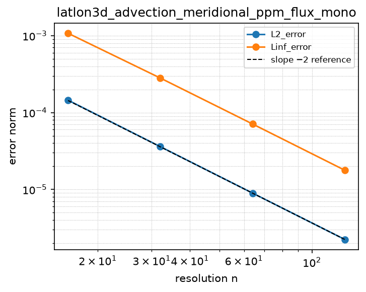
ppm_flux_D_lat_polar
Source: grids/latlon3d/rules/ppm_flux_D_lat_polar.esm
Rewrites ∂(V·q)/∂lat at priority 10 — match pattern:
{"op": "D", "args": [{"op": "*", "args": ["V", "q"]}], "wrt": "lat"}
where): fires only when V is a bare field shaped [lon, lat_nodes, lev]. Under import-edge renaming (§9.7.7) the wrt literal and this shape follow the renamed axis together, so the rule can be imported more than once (each instance scoped to its own grid) without a first-declared-wins collision. A consumer differentiating a compound inline expression must bind it to a declared shaped observed first.Discretization — one makearray tiling the output axes; boundary conditions live in the face regions of this same rule (esm-spec §9.6.8; later regions overwrite earlier, §4.3.2):
| Region | Treatment | Value |
|---|---|---|
lon ∈ [1, NLON], lat ∈ [3, NLAT−2], lev ∈ [1, NLEV] | interior | ppmflux_D_lat_unlim_interior(q, V)[i,j,k] = (ppm_lev_flux(q[i, j−1, k], q[i, j, k], q[i, j+1, k], q[i, j+2, k], dphi_lat[j−1], dphi_lat[j], dphi_lat[j+1], dphi_lat[j+2], V[i, j+1, k])·coslat_e[j+1] − ppm_lev_flux(q[i, j−2, k], q[i, j−1, k], q[i, j, k], q[i, j+1, k], dphi_lat[j−2], dphi_lat[j−1], dphi_lat[j], dphi_lat[j+1], V[i, j, k])·coslat_e[j]) / dS_lat[j] for i ∈ lon, j ∈ [3, NLAT−2], k ∈ lev |
lon ∈ [1, NLON], lat = 1, lev ∈ [1, NLEV] | boundary face | ppmflux_D_lat_unlim_cap_s_j1(q, V)[i,j,k] = (ppm_lev_flux(q[i, 1, k], q[i, 1, k], q[i, 2, k], q[i, 3, k], dphi_lat[1], dphi_lat[1], dphi_lat[2], dphi_lat[3], V[i, 2, k])·coslat_e[2]) / dS_lat[1] for i ∈ lon, j ∈ [1, 1], k ∈ lev |
lon ∈ [1, NLON], lat = 2, lev ∈ [1, NLEV] | boundary face | ppmflux_D_lat_unlim_cap_s_j2(q, V)[i,j,k] = (ppm_lev_flux(q[i, 1, k], q[i, 2, k], q[i, 3, k], q[i, 4, k], dphi_lat[1], dphi_lat[2], dphi_lat[3], dphi_lat[4], V[i, 3, k])·coslat_e[3] − ppm_lev_flux(q[i, 1, k], q[i, 1, k], q[i, 2, k], q[i, 3, k], dphi_lat[1], dphi_lat[1], dphi_lat[2], dphi_lat[3], V[i, 2, k])·coslat_e[2]) / dS_lat[2] for i ∈ lon, j ∈ [2, 2], k ∈ lev |
lon ∈ [1, NLON], lat = NLAT−1, lev ∈ [1, NLEV] | boundary face | ppmflux_D_lat_unlim_cap_n_jNm1(q, V)[i,j,k] = (ppm_lev_flux(q[i, NLAT−2, k], q[i, NLAT−1, k], q[i, NLAT, k], q[i, NLAT, k], dphi_lat[NLAT−2], dphi_lat[NLAT−1], dphi_lat[NLAT], dphi_lat[NLAT], V[i, NLAT, k])·coslat_e[NLAT] − ppm_lev_flux(q[i, NLAT−3, k], q[i, NLAT−2, k], q[i, NLAT−1, k], q[i, NLAT, k], dphi_lat[NLAT−3], dphi_lat[NLAT−2], dphi_lat[NLAT−1], dphi_lat[NLAT], V[i, NLAT−1, k])·coslat_e[NLAT−1]) / dS_lat[NLAT−1] for i ∈ lon, j ∈ [NLAT−1, NLAT−1], k ∈ lev |
lon ∈ [1, NLON], lat = NLAT, lev ∈ [1, NLEV] | boundary face | ppmflux_D_lat_unlim_cap_n_jN(q, V)[i,j,k] = (−(ppm_lev_flux(q[i, NLAT−2, k], q[i, NLAT−1, k], q[i, NLAT, k], q[i, NLAT, k], dphi_lat[NLAT−2], dphi_lat[NLAT−1], dphi_lat[NLAT], dphi_lat[NLAT], V[i, NLAT, k])·coslat_e[NLAT])) / dS_lat[NLAT] for i ∈ lon, j ∈ [NLAT, NLAT], k ∈ lev |
UNLIMITED (CENTRED) CW84 conservative flux-form MERIDIONAL advection D(V*q, wrt: lat) on the latlon3d sphere, with the wind as a MATCHED OPERAND and RIGID POLAR WALLS at both ends. The unlimited sibling of rules/ppm_flux_D_lat_mono_polar: same compound match, same spherical metric, same structurally-omitted pole terms, same free names – only the FACE VALUE differs. It is the meridional rotation of rules/ppm_flux_D_lev_noflux_bc.
THE SCHEME. The face value is the SHARED CW84 eq-(1.6) interpolant of the four rows straddling the face, with NO limiter and NO branch on the sign of the face velocity: F = v * a_{j+1/2} (../stencils/ppm_lev_flux, an axis-neutral atom REUSED here, not cloned). Because the interpolant is shared, both rows see the same face value, the divergence telescopes and mass is conserved exactly – the same guarantee the limited sibling gives.
WHY THERE IS NO ‘UNLIMITED UPWIND’ VARIANT, and why this rule is not simply the mono rule with the limiter switched off. For the UNLIMITED reconstruction the two one-sided face values are IDENTICAL: row j’s parabola and row j+1’s parabola both pass exactly through the shared eq-(1.6) interpolant at the face between them, so there is nothing for an upwind scheme to choose and ‘unlimited upwind PPM’ degenerates term-for-term onto this centred flux. It is the eq (1.10) limiter, applied PER ROW, that pulls row j’s northern endpoint and row j+1’s southern endpoint apart, and only then does the donor choice carry information. Upwind bias is therefore a property of the LIMITED reconstruction, not an independent axis – which is also why this rule’s support is FIVE rows (j-2..j+2, interior [3, NLAT-2], four polar slabs) against the limited sibling’s seven.
SCOPE – THIS IS THE ACCURACY CEILING, NOT THE PRODUCTION OPERATOR. Being centred, the scheme carries NO upwind dissipation: it is stable only where the flow is smooth and the tracer has no sharp gradient, and it will drive a tracer NEGATIVE across a front (the vertical sibling reaches -7.16 on a top-hat plume where the limited one stays at exactly +0.0). Its purpose is to quantify what the limiter costs, and to serve models whose fields are known-smooth. For transport of a chemical tracer, import rules/ppm_flux_D_lat_mono_polar instead.
THE POLE FLUX TERMS ARE STRUCTURALLY OMITTED, exactly as in the limited sibling: at j = 1 the term F_1 coslat_e[1] is ABSENT FROM THE EXPRESSION TREE, and likewise F_{NLAT+1} coslat_e[NLAT+1] at j = NLAT, because cos(-/+pi/2) is 6.1e-17 in IEEE and NOT zero. V[i,1,k] and V[i,NLAT+1,k] are never read. MEASURED with a reversing meridional wind and a random tracer: area-weighted global tendency sum_j dS_lat[j] dq/dt = 4.27e-15 absolute, 4.50e-16 relative – the rounding floor of the summation. Free-stream preservation is likewise BIT-EXACT (every eq-(1.6) correction term is a difference of equal values at q == 1, exactly 0.0 in IEEE, so F = v exactly): verified against the continuity operator rules/face_flux_divergence_lat_polar, max|difference| = 0.0 EXACTLY (0 of 544 cells differ in a single bit) over every cell.
SELECTION IS BY IMPORT. This rule matches the same compound D(Vq, wrt: lat) at the same priority 10 as rules/upwind1_flux_D_lat_polar and rules/ppm_flux_D_lat_mono_polar; a consuming PROBLEM imports exactly ONE. The esm-spec 9.6.1 where shape constraint (not priority) is what keeps the compound match off a meridional diffusion term D(khD(u, wrt: lat), wrt: lat). Requires NLAT >= 5 for a non-empty interior.
FREE NAMES (consumer-supplied): coslat_e [lat_nodes], dS_lat [lat], dphi_lat [lat] – cos(phi_e), the exact spherical cell area, and the cell width in radians, from the grid’s coslat_edge, latcell_area and latcell_dphi. Face j is the SOUTHERN edge of cell j; V is positive NORTHWARD.
MEASURED ORDER ON THIS AXIS IS 2.0, NOT 4.0, AND THE CAUSE IS LOCALISED – READ THIS BEFORE EXPECTING A FOURTH-ORDER OPERATOR. The CW84 reconstruction is formally FOURTH order, and the VERTICAL sibling using the SAME face atom measures a clean 3.99/3.94. On LATITUDE this rule measures L2 1.989 (pairwise 1.979, 1.989, 1.994) / Linf 1.983 (pairwise 1.930, 1.983, 1.996) (convergence case tests/conformance/convergence/latlon3d_advection_meridional_ppm_flux). The shortfall is NOT the limiter – the limited and unlimited lat rules measure the SAME 2.0, and on a smooth field their interior truncation-error fields are BIT-IDENTICAL because the limiter never fires – and it is NOT the nonuniform cap widths. It is TWO independent O(dphi^2) floors, both intrinsic to reconstructing in PHI on a sphere. (1) THE MEASURE MISMATCH, in the interior: the conserved state is the AREA-weighted (sin-weighted) cell mean, which is what the flux form advances, while the parabola is fitted with the widths dphi_lat and so treats the state as a PHI-weighted mean; the two differ by (dphi^2/12) q’ tan(phi), which the reconstruction cannot see. MEASURED DECISIVELY: feeding these SAME stencils dS_lat as the cell width instead of dphi_lat – i.e. reconstructing in mu = sin(phi), where the state IS the exact cell mean – drops the INTERIOR truncation error to MACHINE ZERO (8.0e-15 / 1.6e-14 / 4.7e-14 at NLAT = 17/33/65, against 4.2e-3 / 1.7e-3 / 4.8e-4 as shipped). That experiment also PROVES the stencil wiring exactly correct, since no mis-indexed gather could leave a 1e-14 residual. (2) THE POLAR CAP GHOST CLOSURE: the zero-gradient ghost rows behind each pole are a first-order closure and the half-polar cap divides their error by an O(dphi^2) area; this floor survives even the mu-width experiment, where the cap rows carry the entire remaining error. Every scheme on this axis shows it – the donor-cell rule’s cap rows also converge at exactly 2.00. WHAT THE RECONSTRUCTION BUYS is the CONSTANT and one order: at NLAT = 129 this rule’s L2 is 2.23e-6 (221x better) against the donor cell’s 4.92e-4. Recovering the formal fourth order would mean reconstructing in mu – a one-line change at the CONSUMER’s dphi_lat binding, with no change to any rule or stencil – and is the documented follow-on, deliberately not taken here because this rule’s contract is to replace the donor rule’s FACE FLUX and nothing else.
COMPOSITIONAL BODY: a makearray tiling [lon, lat, lev] with FIVE regions – the interior [3, NLAT-2] uses ../stencils/ppmflux_D_lat_unlim_interior; the south cap rows j = 1,2 use ../stencils/ppmflux_D_lat_unlim_cap_s_j{1,2}; the north cap rows j = NLAT-1, NLAT use ../stencils/ppmflux_D_lat_unlim_cap_n_j{Nm1,N}.
References
- Colella, P., & Woodward, P. R. (1984). The Piecewise Parabolic Method (PPM) for gas-dynamical simulations. Journal of Computational Physics, 54(1), 174-201.
doi:10.1016/0021-9991(84)90143-8 - Lin, S.-J., & Rood, R. B. (1996). Multidimensional flux-form semi-Lagrangian transport schemes. Monthly Weather Review, 124(9), 2046-2070.
doi:10.1175/1520-0493(1996)124<2046:MFFSLT>2.0.CO;2 - Colella, P., & Sekora, M. D. (2008). A limiter for PPM that preserves accuracy at smooth extrema. Journal of Computational Physics, 227(15), 7069-7076.
doi:10.1016/j.jcp.2008.03.034 - LeVeque, R. J. (2002). Finite Volume Methods for Hyperbolic Problems. Cambridge University Press. Section 4.1 (the donor-cell upwind flux; the upwind selection is the same whatever sub-grid reconstruction supplies the two one-sided face values).
- Jacobson, M. Z. (2005). Fundamentals of Atmospheric Modeling (2nd ed.). Cambridge University Press. Chapter 6 (finite-volume flux-form tracer transport; consistency with continuity).
Conformance fixtures
- ast:
latlon3d_ppm_flux_D_lat_polar— statusactive - convergence:
latlon3d_advection_meridional_ppm_flux— statusactive
Convergence — case latlon3d_advection_meridional_ppm_flux
Error norms read from the committed golden tests/conformance/convergence/latlon3d_advection_meridional_ppm_flux/golden/errors.json (binding: julia; nothing recomputed for display).
| n | L2_error | observed order | Linf_error | observed order |
|---|---|---|---|---|
| 16 | 1.391e-04 | — | 1.011e-03 | — |
| 32 | 3.527e-05 | 1.98 | 2.654e-04 | 1.93 |
| 64 | 8.884e-06 | 1.99 | 6.716e-05 | 1.98 |
| 128 | 2.230e-06 | 1.99 | 1.684e-05 | 2.00 |
Expected order: 2 (± 0.15).
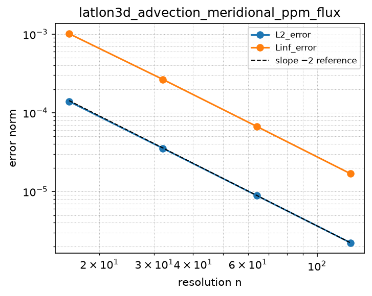
ppm_flux_D_lev_mono_hybrid_noflux_bc
Source: grids/latlon3d/rules/ppm_flux_D_lev_mono_hybrid_noflux_bc.esm
Rewrites ∂(W·q)/∂lev at priority 10 — match pattern:
{"op": "D", "args": [{"op": "*", "args": ["W", "q"]}], "wrt": "lev"}
where): fires only when W is a bare field shaped [lon, lat, lev_nodes]. Under import-edge renaming (§9.7.7) the wrt literal and this shape follow the renamed axis together, so the rule can be imported more than once (each instance scoped to its own grid) without a first-declared-wins collision. A consumer differentiating a compound inline expression must bind it to a declared shaped observed first.Discretization — one makearray tiling the output axes; boundary conditions live in the face regions of this same rule (esm-spec §9.6.8; later regions overwrite earlier, §4.3.2):
| Region | Treatment | Value |
|---|---|---|
lon ∈ [1, NLON], lat ∈ [1, NLAT], lev ∈ [4, NLEV−3] | interior | ppmflux_D_lev_hyb_interior(q, W)[i,j,k] = ppmflux_lev_face_flux(q[i, j, k−2], q[i, j, k−1], q[i, j, k], q[i, j, k+1], q[i, j, k+2], q[i, j, k+3], dp[i, j, k−2], dp[i, j, k−1], dp[i, j, k], dp[i, j, k+1], dp[i, j, k+2], dp[i, j, k+3], W[i, j, k+1]) − ppmflux_lev_face_flux(q[i, j, k−3], q[i, j, k−2], q[i, j, k−1], q[i, j, k], q[i, j, k+1], q[i, j, k+2], dp[i, j, k−3], dp[i, j, k−2], dp[i, j, k−1], dp[i, j, k], dp[i, j, k+1], dp[i, j, k+2], W[i, j, k]) for i ∈ lon, j ∈ lat, k ∈ [4, NLEV−3] |
lon ∈ [1, NLON], lat ∈ [1, NLAT], lev = 1 | boundary face | ppmflux_D_lev_hyb_nf_k1(q, W)[i,j,k] = ppmflux_lev_face_flux(q[i, j, 1], q[i, j, 1], q[i, j, 1], q[i, j, 2], q[i, j, 3], q[i, j, 4], dp[i, j, 1], dp[i, j, 1], dp[i, j, 1], dp[i, j, 2], dp[i, j, 3], dp[i, j, 4], W[i, j, 2]) for i ∈ lon, j ∈ lat, k ∈ [1, 1] |
lon ∈ [1, NLON], lat ∈ [1, NLAT], lev = 2 | boundary face | ppmflux_D_lev_hyb_nf_k2(q, W)[i,j,k] = ppmflux_lev_face_flux(q[i, j, 1], q[i, j, 1], q[i, j, 2], q[i, j, 3], q[i, j, 4], q[i, j, 5], dp[i, j, 1], dp[i, j, 1], dp[i, j, 2], dp[i, j, 3], dp[i, j, 4], dp[i, j, 5], W[i, j, 3]) − ppmflux_lev_face_flux(q[i, j, 1], q[i, j, 1], q[i, j, 1], q[i, j, 2], q[i, j, 3], q[i, j, 4], dp[i, j, 1], dp[i, j, 1], dp[i, j, 1], dp[i, j, 2], dp[i, j, 3], dp[i, j, 4], W[i, j, 2]) for i ∈ lon, j ∈ lat, k ∈ [2, 2] |
lon ∈ [1, NLON], lat ∈ [1, NLAT], lev = 3 | boundary face | ppmflux_D_lev_hyb_nf_k3(q, W)[i,j,k] = ppmflux_lev_face_flux(q[i, j, 1], q[i, j, 2], q[i, j, 3], q[i, j, 4], q[i, j, 5], q[i, j, 6], dp[i, j, 1], dp[i, j, 2], dp[i, j, 3], dp[i, j, 4], dp[i, j, 5], dp[i, j, 6], W[i, j, 4]) − ppmflux_lev_face_flux(q[i, j, 1], q[i, j, 1], q[i, j, 2], q[i, j, 3], q[i, j, 4], q[i, j, 5], dp[i, j, 1], dp[i, j, 1], dp[i, j, 2], dp[i, j, 3], dp[i, j, 4], dp[i, j, 5], W[i, j, 3]) for i ∈ lon, j ∈ lat, k ∈ [3, 3] |
lon ∈ [1, NLON], lat ∈ [1, NLAT], lev = NLEV−2 | boundary face | ppmflux_D_lev_hyb_nf_kNm2(q, W)[i,j,k] = ppmflux_lev_face_flux(q[i, j, NLEV−4], q[i, j, NLEV−3], q[i, j, NLEV−2], q[i, j, NLEV−1], q[i, j, NLEV], q[i, j, NLEV], dp[i, j, NLEV−4], dp[i, j, NLEV−3], dp[i, j, NLEV−2], dp[i, j, NLEV−1], dp[i, j, NLEV], dp[i, j, NLEV], W[i, j, NLEV−1]) − ppmflux_lev_face_flux(q[i, j, NLEV−5], q[i, j, NLEV−4], q[i, j, NLEV−3], q[i, j, NLEV−2], q[i, j, NLEV−1], q[i, j, NLEV], dp[i, j, NLEV−5], dp[i, j, NLEV−4], dp[i, j, NLEV−3], dp[i, j, NLEV−2], dp[i, j, NLEV−1], dp[i, j, NLEV], W[i, j, NLEV−2]) for i ∈ lon, j ∈ lat, k ∈ [NLEV−2, NLEV−2] |
lon ∈ [1, NLON], lat ∈ [1, NLAT], lev = NLEV−1 | boundary face | ppmflux_D_lev_hyb_nf_kNm1(q, W)[i,j,k] = ppmflux_lev_face_flux(q[i, j, NLEV−3], q[i, j, NLEV−2], q[i, j, NLEV−1], q[i, j, NLEV], q[i, j, NLEV], q[i, j, NLEV], dp[i, j, NLEV−3], dp[i, j, NLEV−2], dp[i, j, NLEV−1], dp[i, j, NLEV], dp[i, j, NLEV], dp[i, j, NLEV], W[i, j, NLEV]) − ppmflux_lev_face_flux(q[i, j, NLEV−4], q[i, j, NLEV−3], q[i, j, NLEV−2], q[i, j, NLEV−1], q[i, j, NLEV], q[i, j, NLEV], dp[i, j, NLEV−4], dp[i, j, NLEV−3], dp[i, j, NLEV−2], dp[i, j, NLEV−1], dp[i, j, NLEV], dp[i, j, NLEV], W[i, j, NLEV−1]) for i ∈ lon, j ∈ lat, k ∈ [NLEV−1, NLEV−1] |
lon ∈ [1, NLON], lat ∈ [1, NLAT], lev = NLEV | boundary face | ppmflux_D_lev_hyb_nf_kN(q, W)[i,j,k] = 0 − ppmflux_lev_face_flux(q[i, j, NLEV−3], q[i, j, NLEV−2], q[i, j, NLEV−1], q[i, j, NLEV], q[i, j, NLEV], q[i, j, NLEV], dp[i, j, NLEV−3], dp[i, j, NLEV−2], dp[i, j, NLEV−1], dp[i, j, NLEV], dp[i, j, NLEV], dp[i, j, NLEV], W[i, j, NLEV]) for i ∈ lon, j ∈ lat, k ∈ [NLEV, NLEV] |
UPWIND-BIASED, MONOTONE, conservative flux-form vertical advection for a TERRAIN-FOLLOWING (hybrid sigma-pressure) vertical coordinate whose level thicknesses breathe in time. The moving-grid counterpart of ppm_flux_D_lev_mono_noflux_bc: same seven-region CW84 monotone reconstruction, same matched-operand 3-D face wind, same rigid no-flux walls – but with TWO changes that make it correct and high-order on a grid whose layers move.
MASS FORM (conservative on a moving grid). The fixed-grid rule outputs (F_{k+1/2} - F_{k-1/2}) / dz[k]; dividing by a time-varying cell thickness omits the grid-motion (thickness-tendency) term, so the fixed-grid divergence is conservative ONLY when dz is constant in time and drifts under a breathing surface pressure. This rule instead outputs the RAW face-flux difference F_{k+1/2} - F_{k-1/2} (no division). The consumer writes dmq/dt = -D(W*q, wrt: lev) + … where mq is the cell AIR/TRACER MASS per unit area (a pressure thickness), so the integrated quantity is the extensive cell mass and no moving-grid term is dropped. The horizontal divergence companions (face_flux_divergence_lon/lat, which carry the fixed spherical area measure) combine with this term directly, since on a lat-lon mesh only the vertical coordinate moves.
TERRAIN-FOLLOWING RECONSTRUCTION (high-order on the real thicknesses). The CW84 eq (1.6)/(1.8)/(1.10) parabola is built on the PHYSICAL pressure thicknesses
dp(free name, shape [lon,lat,lev]) – gathered as dp[i,j,k+/-n] over the five-cell window of each endpoint – rather than a 1-D, time-static column dz[k]. On a hybrid grid dp = dA[k] + dB[k]*Ps(i,j,t) varies in longitude, latitude and time, so the sub-grid reconstruction sees the true local layer widths, the Lin-Rood (1996) mass-coordinate reconstruction.
CONSISTENCY WITH CONTINUITY (the property that makes it usable for tracer transport). At q == 1 every CW84 slope is a difference of equal values and is exactly 0.0 in IEEE, so the parabola is the constant 1 REGARDLESS of the breathing widths, each one-sided face value is 1, and the donor flux collapses to F = W bitwise. This operator then reduces to the mass-form vertical continuity difference W_{k+1/2} - W_{k-1/2}; combined with the horizontal continuity companions and a vertical air-mass flux W diagnosed from continuity, a tracer initialised to a uniform mixing ratio stays uniform to the last bit while the layers breathe. This is verified end to end by tests/conformance/simulation/latlon3d_transport_cwc_moving_lid.
SCOPE. Monotone (eq 1.8 + eq 1.10 limiter): bounded, non-negative across sharp vertical gradients, at the documented cost of formal order at smooth extrema (the Colella-Sekora 2008 limiter is the follow-on). Seven-cell support (k-3..k+3): interior [4, NLEV-3], six near-wall slabs, NLEV >= 7 for a non-empty interior. The wind W (the vertical air-mass flux, shape [lon,lat,lev_nodes], positive upward) is a MATCHED OPERAND; W at faces 1 and NLEV+1 is never read (the wall fluxes are absent, not zeroed), so both no-flux walls are exact in floating point. A semi-discrete (method-of-lines) operator, not the fully-discrete TPCORE scheme (see grids/latlon3d/grid.esm SCHEME CAVEAT).
FREE NAME (consumer-supplied): dp, the physical cell pressure thicknesses, shape [lon,lat,lev] (the grid’s lev_thickness_3d contract). The velocity is the matched operand W, NOT a free name.
COMPOSITIONAL BODY: a makearray tiling [lon,lat,lev] with SEVEN regions, each a thin apply of a factored ppmflux_D_lev_hyb_* stencil – interior [4, NLEV-3]; surface cells k = 1,2,3; model-top cells k = NLEV-2, NLEV-1, NLEV. Every region is a full-rank slab aggregate (output_idx [i, j, k]).
References
- Colella, P., & Woodward, P. R. (1984). The Piecewise Parabolic Method (PPM) for gas-dynamical simulations. Journal of Computational Physics, 54(1), 174-201.
doi:10.1016/0021-9991(84)90143-8 - Lin, S.-J., & Rood, R. B. (1996). Multidimensional flux-form semi-Lagrangian transport schemes. Monthly Weather Review, 124(9), 2046-2070.
doi:10.1175/1520-0493(1996)124<2046:MFFSLT>2.0.CO;2 - Colella, P., & Sekora, M. D. (2008). A limiter for PPM that preserves accuracy at smooth extrema. Journal of Computational Physics, 227(15), 7069-7076.
doi:10.1016/j.jcp.2008.03.034 - LeVeque, R. J. (2002). Finite Volume Methods for Hyperbolic Problems. Cambridge University Press. Section 4.1 (the donor-cell upwind flux; the upwind selection is the same whatever sub-grid reconstruction supplies the two one-sided face values).
Conformance fixtures
- ast:
latlon3d_ppm_flux_D_lev_mono_hybrid_noflux_bc— statusactive - simulation:
latlon3d_transport_cwc_moving_lid
ppm_flux_D_lev_mono_noflux_bc
Source: grids/latlon3d/rules/ppm_flux_D_lev_mono_noflux_bc.esm
Rewrites ∂(W·q)/∂lev at priority 10 — match pattern:
{"op": "D", "args": [{"op": "*", "args": ["W", "q"]}], "wrt": "lev"}
where): fires only when W is a bare field shaped [lon, lat, lev_nodes]. Under import-edge renaming (§9.7.7) the wrt literal and this shape follow the renamed axis together, so the rule can be imported more than once (each instance scoped to its own grid) without a first-declared-wins collision. A consumer differentiating a compound inline expression must bind it to a declared shaped observed first.Discretization — one makearray tiling the output axes; boundary conditions live in the face regions of this same rule (esm-spec §9.6.8; later regions overwrite earlier, §4.3.2):
| Region | Treatment | Value |
|---|---|---|
lon ∈ [1, NLON], lat ∈ [1, NLAT], lev ∈ [4, NLEV−3] | interior | ppmflux_D_lev_interior(q, W)[i,j,k] = (ppmflux_lev_face_flux(q[i, j, k−2], q[i, j, k−1], q[i, j, k], q[i, j, k+1], q[i, j, k+2], q[i, j, k+3], dz[k−2], dz[k−1], dz[k], dz[k+1], dz[k+2], dz[k+3], W[i, j, k+1]) − ppmflux_lev_face_flux(q[i, j, k−3], q[i, j, k−2], q[i, j, k−1], q[i, j, k], q[i, j, k+1], q[i, j, k+2], dz[k−3], dz[k−2], dz[k−1], dz[k], dz[k+1], dz[k+2], W[i, j, k])) / dz[k] for i ∈ lon, j ∈ lat, k ∈ [4, NLEV−3] |
lon ∈ [1, NLON], lat ∈ [1, NLAT], lev = 1 | boundary face | ppmflux_D_lev_nf_k1(q, W)[i,j,k] = ppmflux_lev_face_flux(q[i, j, 1], q[i, j, 1], q[i, j, 1], q[i, j, 2], q[i, j, 3], q[i, j, 4], dz[1], dz[1], dz[1], dz[2], dz[3], dz[4], W[i, j, 2]) / dz[1] for i ∈ lon, j ∈ lat, k ∈ [1, 1] |
lon ∈ [1, NLON], lat ∈ [1, NLAT], lev = 2 | boundary face | ppmflux_D_lev_nf_k2(q, W)[i,j,k] = (ppmflux_lev_face_flux(q[i, j, 1], q[i, j, 1], q[i, j, 2], q[i, j, 3], q[i, j, 4], q[i, j, 5], dz[1], dz[1], dz[2], dz[3], dz[4], dz[5], W[i, j, 3]) − ppmflux_lev_face_flux(q[i, j, 1], q[i, j, 1], q[i, j, 1], q[i, j, 2], q[i, j, 3], q[i, j, 4], dz[1], dz[1], dz[1], dz[2], dz[3], dz[4], W[i, j, 2])) / dz[2] for i ∈ lon, j ∈ lat, k ∈ [2, 2] |
lon ∈ [1, NLON], lat ∈ [1, NLAT], lev = 3 | boundary face | ppmflux_D_lev_nf_k3(q, W)[i,j,k] = (ppmflux_lev_face_flux(q[i, j, 1], q[i, j, 2], q[i, j, 3], q[i, j, 4], q[i, j, 5], q[i, j, 6], dz[1], dz[2], dz[3], dz[4], dz[5], dz[6], W[i, j, 4]) − ppmflux_lev_face_flux(q[i, j, 1], q[i, j, 1], q[i, j, 2], q[i, j, 3], q[i, j, 4], q[i, j, 5], dz[1], dz[1], dz[2], dz[3], dz[4], dz[5], W[i, j, 3])) / dz[3] for i ∈ lon, j ∈ lat, k ∈ [3, 3] |
lon ∈ [1, NLON], lat ∈ [1, NLAT], lev = NLEV−2 | boundary face | ppmflux_D_lev_nf_kNm2(q, W)[i,j,k] = (ppmflux_lev_face_flux(q[i, j, NLEV−4], q[i, j, NLEV−3], q[i, j, NLEV−2], q[i, j, NLEV−1], q[i, j, NLEV], q[i, j, NLEV], dz[NLEV−4], dz[NLEV−3], dz[NLEV−2], dz[NLEV−1], dz[NLEV], dz[NLEV], W[i, j, NLEV−1]) − ppmflux_lev_face_flux(q[i, j, NLEV−5], q[i, j, NLEV−4], q[i, j, NLEV−3], q[i, j, NLEV−2], q[i, j, NLEV−1], q[i, j, NLEV], dz[NLEV−5], dz[NLEV−4], dz[NLEV−3], dz[NLEV−2], dz[NLEV−1], dz[NLEV], W[i, j, NLEV−2])) / dz[NLEV−2] for i ∈ lon, j ∈ lat, k ∈ [NLEV−2, NLEV−2] |
lon ∈ [1, NLON], lat ∈ [1, NLAT], lev = NLEV−1 | boundary face | ppmflux_D_lev_nf_kNm1(q, W)[i,j,k] = (ppmflux_lev_face_flux(q[i, j, NLEV−3], q[i, j, NLEV−2], q[i, j, NLEV−1], q[i, j, NLEV], q[i, j, NLEV], q[i, j, NLEV], dz[NLEV−3], dz[NLEV−2], dz[NLEV−1], dz[NLEV], dz[NLEV], dz[NLEV], W[i, j, NLEV]) − ppmflux_lev_face_flux(q[i, j, NLEV−4], q[i, j, NLEV−3], q[i, j, NLEV−2], q[i, j, NLEV−1], q[i, j, NLEV], q[i, j, NLEV], dz[NLEV−4], dz[NLEV−3], dz[NLEV−2], dz[NLEV−1], dz[NLEV], dz[NLEV], W[i, j, NLEV−1])) / dz[NLEV−1] for i ∈ lon, j ∈ lat, k ∈ [NLEV−1, NLEV−1] |
lon ∈ [1, NLON], lat ∈ [1, NLAT], lev = NLEV | boundary face | ppmflux_D_lev_nf_kN(q, W)[i,j,k] = (0 − ppmflux_lev_face_flux(q[i, j, NLEV−3], q[i, j, NLEV−2], q[i, j, NLEV−1], q[i, j, NLEV], q[i, j, NLEV], q[i, j, NLEV], dz[NLEV−3], dz[NLEV−2], dz[NLEV−1], dz[NLEV], dz[NLEV], dz[NLEV], W[i, j, NLEV])) / dz[NLEV] for i ∈ lon, j ∈ lat, k ∈ [NLEV, NLEV] |
UPWIND-BIASED, MONOTONE, conservative flux-form vertical advection d/dz(w q) on the latlon3d stretched vertical, with the wind as a MATCHED OPERAND and rigid no-flux walls at the surface and the model top. THE PRODUCTION VERTICAL TRANSPORT OPERATOR ON THIS GRID: it is the only one that is simultaneously high-order, mass-conserving, bounded, and correct for a wind that reverses sign. A consuming model writes du/dt = -D(W*u, wrt: lev) + … and this rule lowers the whole compound.
WHAT IT COMBINES, AND THE GAP IT CLOSES. The library previously offered two half-answers. rules/upwind1_flux_D_lev_noflux_bc takes a genuine 3-D face-staggered wind and can SEE the sign of the face velocity, so it upwinds correctly through a reversal – but its face value is the first-order DONOR CELL value, O(dz) and far too diffusive to carry a plume. rules/ppm_D_lev_mono_noflux_bc reconstructs a third/fourth-order CW84 parabola – but it matches a BARE D(f, wrt: lev), reads its velocity from a free name w_edge of shape [lev_nodes] (a 1-D, k-only, time-static column profile), and its face value is the CENTRED eq-(1.6) interpolant with NO branch on the sign of w, so it is not upwind-biased at all and is correct only for a one-signed wind. This rule is their join: the compound match and 3-D matched-operand wind of the former, the high-order limited reconstruction of the latter, and a genuine sign-of-w donor selection between them.
THE SCHEME. At each face PPM supplies TWO one-sided values: aR_L, the LEFT (lower) cell’s limited parabola at its own upper endpoint, and aL_R, the RIGHT (upper) cell’s limited parabola at its own lower endpoint. The flux donates from the cell the flow comes FROM: F = waR_L for w > 0 and waL_R for w < 0, spelled branch-free as F = max(w,0)*aR_L + min(w,0)*aL_R (../stencils/ppmflux_lev_face_flux, which explains why that form is preferred over the textbook 1/2[w(aR_L+aL_R) - |w|(aL_R-aR_L)]: it mentions each multi-megabyte reconstruction once rather than twice, and it returns the donor flux EXACTLY in floating point). Both endpoints carry the full CW84 chain – eq (1.6) edge interpolation on eq (1.8) monotonized slopes, then the eq (1.10) parabola limiter (../stencils/ppmflux_lev_cell_aR and ppmflux_lev_cell_aL, over ppm_lev_edge_mono, ppm_limit_right and the new mirror ppmflux_limit_left).
WHY UPWIND BIAS AND LIMITING ARE INSEPARABLE – the non-obvious fact this rule is built on. For the UNLIMITED reconstruction the two one-sided face values are IDENTICAL: cell j’s parabola and cell j+1’s parabola both pass exactly through the shared eq-(1.6) interpolant at the face between them, so there is nothing for an upwind scheme to choose and ‘unlimited upwind PPM’ degenerates term-for-term onto the centred flux of the sibling rules/ppm_flux_D_lev_noflux_bc. It is the eq (1.10) limiter, applied PER CELL, that pulls cell j’s upper endpoint and cell j+1’s lower endpoint apart – each is clipped against its own average and its own far edge – and only then does the donor choice carry information. Upwind-biased PPM is therefore a property of the LIMITED reconstruction, not an independent axis.
COST OF THE BIAS: SEVEN CELLS, SIX BOUNDARY SLABS. Asking a face for BOTH neighbours’ endpoints (rather than only the upwind one, as the pre-existing mono chain does under its hard-coded upward wind) widens the divergence support from six cells to seven (k-3..k+3), so the interior is [4, NLEV-3] and there are six near-wall slabs instead of five. Requires NLEV >= 6 to tile and NLEV >= 7 for a non-empty interior.
BOUNDEDNESS AND ORDER. The eq (1.8) + eq (1.10) limiter pair keeps the reconstruction within the range of the neighbouring cell averages, so the scheme introduces no new extrema and keeps a chemical tracer NON-NEGATIVE across a sharp vertical gradient – a capping inversion, a stack plume, the tropopause ozone jump. That is not a theoretical nicety: the unlimited chain measurably drives such a profile negative, and negative concentrations propagate into the chemistry and aerosol-thermodynamics solvers, while the usual field fix (clipping to zero) silently destroys the exact mass conservation the flux form exists to provide. The price is formal order: a limiter cannot distinguish a smooth extremum from an oscillation and clips it. MEASURED on the manufactured solution of problems/latlon3d_advection_vertical_ppm_flux_mono: L2 2.49, Linf 1.98 – against the 3.99 / 3.94 the unlimited sibling measures on the IDENTICAL MMS, which localises the entire shortfall to the limiter (u*(z) = cos(pi z) has a smooth extremum sitting exactly on the surface wall, so the limiter fires there on every mesh however fine). VERIFIED BOUNDEDNESS, not assumed: on a sharp top-hat plume driven by a reversing, convergent wind the tracer minimum over the whole trajectory is exactly +0.0 under this rule, while the unlimited sibling reaches -7.16 and the pre-existing one-signed ppm_D_lev_mono_noflux_bc – which reconstructs from the DOWNWIND side wherever w < 0, outside its documented w >= 0 contract – diverges to -1.6e3. Mass is conserved to machine zero (relative drift 2.3e-15) in every case. That is the deliberate trade – order you cannot realize on a real vertical profile, exchanged for boundedness you always need. The extremum-preserving Colella-Sekora (2008) limiter is the documented follow-on that would recover it.
THE MATCH IS SHARED WITH ITS ACCURACY SIBLINGS, DELIBERATELY. This rule matches the same compound D(W*q, wrt: lev) as rules/upwind1_flux_D_lev_noflux_bc (first-order donor cell) and as the other member of this pair. They are accuracy siblings over one contract, exactly as the pre-existing ppm_D_lev_noflux_bc and ppm_D_lev_mono_noflux_bc both match a bare D(f, wrt: lev) and coexist. A consuming PROBLEM imports exactly ONE of them; there is no priority game to arbitrate between them and none is wanted.
WHY THE COMPOUND MATCH CANNOT COLLIDE WITH THE DIFFUSION RULE (as for upwind1_flux_D_lev_noflux_bc): a model carrying vertical diffusion contains D(kz*D(u, wrt: lev), wrt: lev), whose outer node is also a D of a two-factor product, so this pattern structurally matches it too, binding W := kz and q := D(u, wrt: lev). It is the where SHAPE CONSTRAINT, not priority, that separates them: by esm-spec 9.6.1 a shape constraint is satisfied only when the bound sub-AST is a bare variable-reference string, and the compound D(u, wrt: lev) fails it, so this rule is filtered out at that node before any priority selection runs. Advection and diffusion therefore compose in one equation, each firing on its own term. Matching is STRUCTURAL and NON-COMMUTATIVE: the velocity must be written on the LEFT of the product.
FREE NAMES (consumer-supplied): dz, the cell thicknesses (the grid’s lev_thickness contract, shape [lev]). The velocity is NOT a free name – it is the matched operand W, of shape [lon, lat, lev_nodes], face-staggered and positive UPWARD. Face k is the lower edge of cell k; W[.,.,1] (ground) and W[.,.,NLEV+1] (model top) are never read, because the wall fluxes are literally absent from the k=1 and k=NLEV slabs rather than formed and multiplied by zero. Mass is therefore conserved to the bit regardless of what the consumer stores in those two faces.
A semi-discrete (method-of-lines) flux-form scheme is NOT the fully-discrete flux-form semi-Lagrangian TPCORE scheme of Lin & Rood (1996) that GEOS-Chem runs operationally: TPCORE carries the Courant number inside the operator and cannot be expressed method-of-lines (see the SCHEME CAVEAT in grids/latlon3d/grid.esm).
COMPOSITIONAL BODY: a makearray tiling [lon, lat, lev] with SEVEN regions, each a thin apply of a factored stencil – the interior [4, NLEV-3] uses ../stencils/ppmflux_D_lev_interior; the surface cells k = 1,2,3 use ../stencils/ppmflux_D_lev_nf_k{1,2,3}; the model-top cells k = NLEV-2, NLEV-1, NLEV use ../stencils/ppmflux_D_lev_nf_k{Nm2,Nm1,N}. Every region is a full-rank slab aggregate (output_idx [i, j, k]).
References
- Colella, P., & Woodward, P. R. (1984). The Piecewise Parabolic Method (PPM) for gas-dynamical simulations. Journal of Computational Physics, 54(1), 174-201.
doi:10.1016/0021-9991(84)90143-8 - Lin, S.-J., & Rood, R. B. (1996). Multidimensional flux-form semi-Lagrangian transport schemes. Monthly Weather Review, 124(9), 2046-2070.
doi:10.1175/1520-0493(1996)124<2046:MFFSLT>2.0.CO;2 - Colella, P., & Sekora, M. D. (2008). A limiter for PPM that preserves accuracy at smooth extrema. Journal of Computational Physics, 227(15), 7069-7076.
doi:10.1016/j.jcp.2008.03.034 - LeVeque, R. J. (2002). Finite Volume Methods for Hyperbolic Problems. Cambridge University Press. Section 4.1 (the donor-cell upwind flux; the upwind selection is the same whatever sub-grid reconstruction supplies the two one-sided face values).
Conformance fixtures
- ast:
latlon3d_ppm_flux_D_lev_mono_noflux_bc— statusactive - convergence:
latlon3d_advection_vertical_ppm_flux_mono— statusactive - simulation:
latlon3d_transport_cwc_3d_ppm
Convergence — case latlon3d_advection_vertical_ppm_flux_mono
Error norms read from the committed golden tests/conformance/convergence/latlon3d_advection_vertical_ppm_flux_mono/golden/errors.json (binding: julia; nothing recomputed for display).
| n | L2_error | observed order | Linf_error | observed order |
|---|---|---|---|---|
| 16 | 5.052e-03 | — | 1.415e-02 | — |
| 32 | 9.074e-04 | 2.48 | 3.705e-03 | 1.93 |
| 64 | 1.613e-04 | 2.49 | 9.413e-04 | 1.98 |
| 128 | 2.859e-05 | 2.50 | 2.368e-04 | 1.99 |
Expected order: 2.24 (± 0.3).
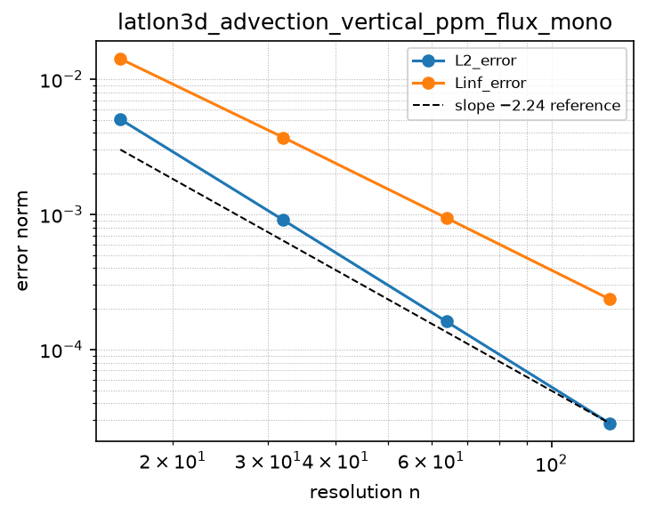
ppm_flux_D_lev_noflux_bc
Source: grids/latlon3d/rules/ppm_flux_D_lev_noflux_bc.esm
Rewrites ∂(W·q)/∂lev at priority 10 — match pattern:
{"op": "D", "args": [{"op": "*", "args": ["W", "q"]}], "wrt": "lev"}
where): fires only when W is a bare field shaped [lon, lat, lev_nodes]. Under import-edge renaming (§9.7.7) the wrt literal and this shape follow the renamed axis together, so the rule can be imported more than once (each instance scoped to its own grid) without a first-declared-wins collision. A consumer differentiating a compound inline expression must bind it to a declared shaped observed first.Discretization — one makearray tiling the output axes; boundary conditions live in the face regions of this same rule (esm-spec §9.6.8; later regions overwrite earlier, §4.3.2):
| Region | Treatment | Value |
|---|---|---|
lon ∈ [1, NLON], lat ∈ [1, NLAT], lev ∈ [3, NLEV−2] | interior | ppmflux_D_lev_unlim_interior(q, W)[i,j,k] = (ppm_lev_flux(q[i, j, k−1], q[i, j, k], q[i, j, k+1], q[i, j, k+2], dz[k−1], dz[k], dz[k+1], dz[k+2], W[i, j, k+1]) − ppm_lev_flux(q[i, j, k−2], q[i, j, k−1], q[i, j, k], q[i, j, k+1], dz[k−2], dz[k−1], dz[k], dz[k+1], W[i, j, k])) / dz[k] for i ∈ lon, j ∈ lat, k ∈ [3, NLEV−2] |
lon ∈ [1, NLON], lat ∈ [1, NLAT], lev = 1 | boundary face | ppmflux_D_lev_unlim_nf_k1(q, W)[i,j,k] = ppm_lev_flux(q[i, j, 1], q[i, j, 1], q[i, j, 2], q[i, j, 3], dz[1], dz[1], dz[2], dz[3], W[i, j, 2]) / dz[1] for i ∈ lon, j ∈ lat, k ∈ [1, 1] |
lon ∈ [1, NLON], lat ∈ [1, NLAT], lev = 2 | boundary face | ppmflux_D_lev_unlim_nf_k2(q, W)[i,j,k] = (ppm_lev_flux(q[i, j, 1], q[i, j, 2], q[i, j, 3], q[i, j, 4], dz[1], dz[2], dz[3], dz[4], W[i, j, 3]) − ppm_lev_flux(q[i, j, 1], q[i, j, 1], q[i, j, 2], q[i, j, 3], dz[1], dz[1], dz[2], dz[3], W[i, j, 2])) / dz[2] for i ∈ lon, j ∈ lat, k ∈ [2, 2] |
lon ∈ [1, NLON], lat ∈ [1, NLAT], lev = NLEV−1 | boundary face | ppmflux_D_lev_unlim_nf_kNm1(q, W)[i,j,k] = (ppm_lev_flux(q[i, j, NLEV−2], q[i, j, NLEV−1], q[i, j, NLEV], q[i, j, NLEV], dz[NLEV−2], dz[NLEV−1], dz[NLEV], dz[NLEV], W[i, j, NLEV]) − ppm_lev_flux(q[i, j, NLEV−3], q[i, j, NLEV−2], q[i, j, NLEV−1], q[i, j, NLEV], dz[NLEV−3], dz[NLEV−2], dz[NLEV−1], dz[NLEV], W[i, j, NLEV−1])) / dz[NLEV−1] for i ∈ lon, j ∈ lat, k ∈ [NLEV−1, NLEV−1] |
lon ∈ [1, NLON], lat ∈ [1, NLAT], lev = NLEV | boundary face | ppmflux_D_lev_unlim_nf_kN(q, W)[i,j,k] = (0 − ppm_lev_flux(q[i, j, NLEV−2], q[i, j, NLEV−1], q[i, j, NLEV], q[i, j, NLEV], dz[NLEV−2], dz[NLEV−1], dz[NLEV], dz[NLEV], W[i, j, NLEV])) / dz[NLEV] for i ∈ lon, j ∈ lat, k ∈ [NLEV, NLEV] |
UNLIMITED (centred) fourth-order CW84 conservative flux-form vertical advection d/dz(w q) on the latlon3d stretched vertical, with the wind as a MATCHED OPERAND and rigid no-flux walls at the surface and the model top. The high-order, non-dissipative ACCURACY CEILING of this family; its bounded, upwind-biased production sibling is rules/ppm_flux_D_lev_mono_noflux_bc. A consuming model writes du/dt = -D(W*u, wrt: lev) + … and this rule lowers the whole compound.
WHAT IS NEW relative to the pre-existing rules/ppm_D_lev_noflux_bc, which computes the IDENTICAL face value: the velocity, and therefore the conservation guarantee. The pre-existing rule matches a BARE D(f, wrt: lev) and reads its velocity from the free name w_edge, a 1-D, k-only, time-static column profile of shape [lev_nodes]; the consuming model cannot hand it a real wind. This rule matches the COMPOUND D(Wq, wrt: lev) with W of shape [lon, lat, lev_nodes] – a genuine three-dimensional, face-staggered wind of the kind a meteorological field supplies – and differences the PRODUCT Wq at faces, so tracer mass telescopes exactly for ANY wind field rather than only for a constant one.
IT IS CENTRED, NOT UPWIND-BIASED, AND THAT IS A THEOREM RATHER THAN AN OMISSION. Its face value is the shared CW84 eq-(1.6) interface interpolant, which does not consult the sign of w. One might expect an upwind-biased variant of it, but there is none to build: for the UNLIMITED reconstruction the parabola of the cell below a face and the parabola of the cell above it pass through EXACTLY the same value at that face, so the two one-sided donor values coincide identically and the donor choice is vacuous – an ‘unlimited upwind PPM’ collapses, term for term, back onto this rule. Upwind bias acquires content only once the eq (1.10) limiter has pulled the two cells’ endpoints apart, which is precisely what the monotone sibling does. USE THIS RULE when the vertical field is smooth and the fourth order is wanted (and as the accuracy ceiling the monotone sibling is measured against); use the monotone sibling for a real tracer, because a centred flux overshoots at a sharp gradient and will drive a concentration negative.
Support is five cells (k-2..k+2): the interior [3, NLEV-2] uses ../stencils/ppmflux_D_lev_unlim_interior over the pre-existing ../stencils/ppm_lev_flux (eq (1.6) edge on raw eq (1.7) slopes -> ppm_lev_edge -> ppm_lev_edge_core + ppm_lev_slope), and the four near-wall cells k = 1, 2, NLEV-1, NLEV use ../stencils/ppmflux_D_lev_unlim_nf_k{1,2,Nm1,N}. Requires NLEV >= 4 to tile.
THE MATCH IS SHARED WITH ITS ACCURACY SIBLINGS, DELIBERATELY. This rule matches the same compound D(W*q, wrt: lev) as rules/upwind1_flux_D_lev_noflux_bc (first-order donor cell) and as the other member of this pair. They are accuracy siblings over one contract, exactly as the pre-existing ppm_D_lev_noflux_bc and ppm_D_lev_mono_noflux_bc both match a bare D(f, wrt: lev) and coexist. A consuming PROBLEM imports exactly ONE of them; there is no priority game to arbitrate between them and none is wanted.
WHY THE COMPOUND MATCH CANNOT COLLIDE WITH THE DIFFUSION RULE (as for upwind1_flux_D_lev_noflux_bc): a model carrying vertical diffusion contains D(kz*D(u, wrt: lev), wrt: lev), whose outer node is also a D of a two-factor product, so this pattern structurally matches it too, binding W := kz and q := D(u, wrt: lev). It is the where SHAPE CONSTRAINT, not priority, that separates them: by esm-spec 9.6.1 a shape constraint is satisfied only when the bound sub-AST is a bare variable-reference string, and the compound D(u, wrt: lev) fails it, so this rule is filtered out at that node before any priority selection runs. Advection and diffusion therefore compose in one equation, each firing on its own term. Matching is STRUCTURAL and NON-COMMUTATIVE: the velocity must be written on the LEFT of the product.
FREE NAMES (consumer-supplied): dz, the cell thicknesses (the grid’s lev_thickness contract, shape [lev]). The velocity is NOT a free name – it is the matched operand W, of shape [lon, lat, lev_nodes], face-staggered and positive UPWARD. Face k is the lower edge of cell k; W[.,.,1] (ground) and W[.,.,NLEV+1] (model top) are never read, because the wall fluxes are literally absent from the k=1 and k=NLEV slabs rather than formed and multiplied by zero. Mass is therefore conserved to the bit regardless of what the consumer stores in those two faces.
A semi-discrete (method-of-lines) flux-form scheme is NOT the fully-discrete flux-form semi-Lagrangian TPCORE scheme of Lin & Rood (1996) that GEOS-Chem runs operationally: TPCORE carries the Courant number inside the operator and cannot be expressed method-of-lines (see the SCHEME CAVEAT in grids/latlon3d/grid.esm).
COMPOSITIONAL BODY: a makearray tiling [lon, lat, lev] with FIVE regions, each a thin apply of a factored stencil. Every region is a full-rank slab aggregate (output_idx [i, j, k]).
References
- Colella, P., & Woodward, P. R. (1984). The Piecewise Parabolic Method (PPM) for gas-dynamical simulations. Journal of Computational Physics, 54(1), 174-201.
doi:10.1016/0021-9991(84)90143-8 - Lin, S.-J., & Rood, R. B. (1996). Multidimensional flux-form semi-Lagrangian transport schemes. Monthly Weather Review, 124(9), 2046-2070.
doi:10.1175/1520-0493(1996)124<2046:MFFSLT>2.0.CO;2
Conformance fixtures
- ast:
latlon3d_ppm_flux_D_lev_noflux_bc— statusactive - convergence:
latlon3d_advection_vertical_ppm_flux— statusactive
Convergence — case latlon3d_advection_vertical_ppm_flux
Error norms read from the committed golden tests/conformance/convergence/latlon3d_advection_vertical_ppm_flux/golden/errors.json (binding: julia; nothing recomputed for display).
| n | L2_error | observed order | Linf_error | observed order |
|---|---|---|---|---|
| 16 | 4.525e-05 | — | 9.648e-05 | — |
| 32 | 2.899e-06 | 3.96 | 6.653e-06 | 3.86 |
| 64 | 1.822e-07 | 3.99 | 4.335e-07 | 3.94 |
| 128 | 1.140e-08 | 4.00 | 2.761e-08 | 3.97 |
Expected order: 4 (± 0.15).
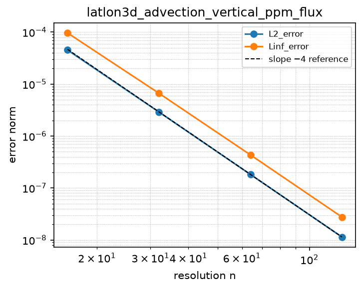
ppm_flux_D_lon_mono_inflow_bc
Source: grids/latlon3d/rules/ppm_flux_D_lon_mono_inflow_bc.esm
Rewrites D(U·q, qbc_w, qbc_e) at priority 10 — match pattern:
{"op": "D", "args": [{"op": "*", "args": ["U", "q"]}, "qbc_w", "qbc_e"], "wrt": "lon"}
where): fires only when U is a bare field shaped [lon_nodes, lat, lev]. Under import-edge renaming (§9.7.7) the wrt literal and this shape follow the renamed axis together, so the rule can be imported more than once (each instance scoped to its own grid) without a first-declared-wins collision. A consumer differentiating a compound inline expression must bind it to a declared shaped observed first.Discretization — one makearray tiling the output axes; boundary conditions live in the face regions of this same rule (esm-spec §9.6.8; later regions overwrite earlier, §4.3.2):
| Region | Treatment | Value |
|---|---|---|
lon ∈ [4, NLON−3], lat ∈ [1, NLAT], lev ∈ [1, NLEV] | interior | ppmflux_D_lon_interior(q, U)[i,j,k] = (dphi_lat[j] / ((dlon_deg·(3.14159265359 / 180))·dS_lat[j]))·(ppmflux_lev_face_flux(q[i−2, j, k], q[i−1, j, k], q[i, j, k], q[i+1, j, k], q[i+2, j, k], q[i+3, j, k], dlon_deg, dlon_deg, dlon_deg, dlon_deg, dlon_deg, dlon_deg, U[i+1, j, k]) − ppmflux_lev_face_flux(q[i−3, j, k], q[i−2, j, k], q[i−1, j, k], q[i, j, k], q[i+1, j, k], q[i+2, j, k], dlon_deg, dlon_deg, dlon_deg, dlon_deg, dlon_deg, dlon_deg, U[i, j, k])) for i ∈ [4, NLON−3], j ∈ lat, k ∈ lev |
lon = 1, lat ∈ [1, NLAT], lev ∈ [1, NLEV] | boundary face | ppmflux_D_lon_inflow_i1(q, U, qbc_w)[i,j,k] = (dphi_lat[j] / ((dlon_deg·(3.14159265359 / 180))·dS_lat[j]))·(ppmflux_lev_face_flux(qbc_w[j, k], qbc_w[j, k], q[1, j, k], q[2, j, k], q[3, j, k], q[4, j, k], dlon_deg, dlon_deg, dlon_deg, dlon_deg, dlon_deg, dlon_deg, U[2, j, k]) − ppmflux_lev_face_flux(qbc_w[j, k], qbc_w[j, k], qbc_w[j, k], q[1, j, k], q[2, j, k], q[3, j, k], dlon_deg, dlon_deg, dlon_deg, dlon_deg, dlon_deg, dlon_deg, U[1, j, k])) for i ∈ [1, 1], j ∈ lat, k ∈ lev |
lon = 2, lat ∈ [1, NLAT], lev ∈ [1, NLEV] | boundary face | ppmflux_D_lon_inflow_i2(q, U, qbc_w)[i,j,k] = (dphi_lat[j] / ((dlon_deg·(3.14159265359 / 180))·dS_lat[j]))·(ppmflux_lev_face_flux(qbc_w[j, k], q[1, j, k], q[2, j, k], q[3, j, k], q[4, j, k], q[5, j, k], dlon_deg, dlon_deg, dlon_deg, dlon_deg, dlon_deg, dlon_deg, U[3, j, k]) − ppmflux_lev_face_flux(qbc_w[j, k], qbc_w[j, k], q[1, j, k], q[2, j, k], q[3, j, k], q[4, j, k], dlon_deg, dlon_deg, dlon_deg, dlon_deg, dlon_deg, dlon_deg, U[2, j, k])) for i ∈ [2, 2], j ∈ lat, k ∈ lev |
lon = 3, lat ∈ [1, NLAT], lev ∈ [1, NLEV] | boundary face | ppmflux_D_lon_inflow_i3(q, U, qbc_w)[i,j,k] = (dphi_lat[j] / ((dlon_deg·(3.14159265359 / 180))·dS_lat[j]))·(ppmflux_lev_face_flux(q[1, j, k], q[2, j, k], q[3, j, k], q[4, j, k], q[5, j, k], q[6, j, k], dlon_deg, dlon_deg, dlon_deg, dlon_deg, dlon_deg, dlon_deg, U[4, j, k]) − ppmflux_lev_face_flux(qbc_w[j, k], q[1, j, k], q[2, j, k], q[3, j, k], q[4, j, k], q[5, j, k], dlon_deg, dlon_deg, dlon_deg, dlon_deg, dlon_deg, dlon_deg, U[3, j, k])) for i ∈ [3, 3], j ∈ lat, k ∈ lev |
lon = NLON−2, lat ∈ [1, NLAT], lev ∈ [1, NLEV] | boundary face | ppmflux_D_lon_inflow_iNm2(q, U, qbc_e)[i,j,k] = (dphi_lat[j] / ((dlon_deg·(3.14159265359 / 180))·dS_lat[j]))·(ppmflux_lev_face_flux(q[NLON−4, j, k], q[NLON−3, j, k], q[NLON−2, j, k], q[NLON−1, j, k], q[NLON, j, k], qbc_e[j, k], dlon_deg, dlon_deg, dlon_deg, dlon_deg, dlon_deg, dlon_deg, U[NLON−1, j, k]) − ppmflux_lev_face_flux(q[NLON−5, j, k], q[NLON−4, j, k], q[NLON−3, j, k], q[NLON−2, j, k], q[NLON−1, j, k], q[NLON, j, k], dlon_deg, dlon_deg, dlon_deg, dlon_deg, dlon_deg, dlon_deg, U[NLON−2, j, k])) for i ∈ [NLON−2, NLON−2], j ∈ lat, k ∈ lev |
lon = NLON−1, lat ∈ [1, NLAT], lev ∈ [1, NLEV] | boundary face | ppmflux_D_lon_inflow_iNm1(q, U, qbc_e)[i,j,k] = (dphi_lat[j] / ((dlon_deg·(3.14159265359 / 180))·dS_lat[j]))·(ppmflux_lev_face_flux(q[NLON−3, j, k], q[NLON−2, j, k], q[NLON−1, j, k], q[NLON, j, k], qbc_e[j, k], qbc_e[j, k], dlon_deg, dlon_deg, dlon_deg, dlon_deg, dlon_deg, dlon_deg, U[NLON, j, k]) − ppmflux_lev_face_flux(q[NLON−4, j, k], q[NLON−3, j, k], q[NLON−2, j, k], q[NLON−1, j, k], q[NLON, j, k], qbc_e[j, k], dlon_deg, dlon_deg, dlon_deg, dlon_deg, dlon_deg, dlon_deg, U[NLON−1, j, k])) for i ∈ [NLON−1, NLON−1], j ∈ lat, k ∈ lev |
lon = NLON, lat ∈ [1, NLAT], lev ∈ [1, NLEV] | boundary face | ppmflux_D_lon_inflow_iN(q, U, qbc_e)[i,j,k] = (dphi_lat[j] / ((dlon_deg·(3.14159265359 / 180))·dS_lat[j]))·(ppmflux_lev_face_flux(q[NLON−2, j, k], q[NLON−1, j, k], q[NLON, j, k], qbc_e[j, k], qbc_e[j, k], qbc_e[j, k], dlon_deg, dlon_deg, dlon_deg, dlon_deg, dlon_deg, dlon_deg, U[NLON+1, j, k]) − ppmflux_lev_face_flux(q[NLON−3, j, k], q[NLON−2, j, k], q[NLON−1, j, k], q[NLON, j, k], qbc_e[j, k], qbc_e[j, k], dlon_deg, dlon_deg, dlon_deg, dlon_deg, dlon_deg, dlon_deg, U[NLON, j, k])) for i ∈ [NLON, NLON], j ∈ lat, k ∈ lev |
UPWIND-BIASED, MONOTONE, conservative flux-form ZONAL advection D(Uq, wrt: lon) on the latlon3d grid for a REGIONAL (limited-area) domain with OPEN lateral boundaries: a prescribed lateral-boundary concentration (Dirichlet inflow) carried in through whichever wall the wind blows INTO, and the interior reconstruction carried out through whichever wall it blows OUT of. The open-boundary sibling of rules/ppm_flux_D_lon_mono_periodic: identical interior, identical spherical metric, identical CW84 eq (1.6)/(1.8)/(1.10) limited reconstruction and sign-of-velocity donor selection (../stencils/ppmflux_lev_face_flux), and the SAME seven-cell support – only the boundary closure differs. The periodic rule ROTATES the ghost indices around the zonal circle; this rule FORMS each open wall flux from a prescribed exterior halo instead. THE HALO IS THE BOUNDARY RECONSTRUCTION (full order, not donor). Near each wall the seven-cell reconstruction reaches for out-of-domain cells; those are supplied by the boundary concentrations qbc_w (west, shape [lat, lev]) and qbc_e (east), a constant halo along the wall at each level, passed as OPERANDS of the matched derivative. The wall face flux is then the CW84-limited one-sided reconstruction over that halo, upwind-selected: F = max(w,0)aR_ext + min(w,0)aL_int, so on INFLOW (w into the domain) the prescribed halo is donated and on OUTFLOW the interior parabola leaves. Each of the two walls handles BOTH regimes by the sign of the wall-normal wind – strictly more general than the 1-D grids/cartesian_uniform_1d/rules/ppm_D_inflow_bc, which hard-codes one inflow wall and one outflow wall for a one-signed speed. CONSISTENCY WITH CONTINUITY / FREE-STREAM. At q == 1 with the halo == 1, every CW84 correction term is a difference of equal values and is exactly 0.0 in IEEE, each parabola is the constant 1, every wall flux collapses to F = w exactly, and the tendency is BITWISE the pure mass divergence: a tracer carried as mq alongside the air mass m stays exactly equal through the open walls (gated by tests/conformance/simulation/latlon3d_transport_cwc_regional_inflow). CONSERVATION. Every INTERIOR interface face is built from the SAME atom, cells, widths and face velocity in the two cells that share it (the boundary slabs are ../stencils/ppmflux_D_lon_interior with only the out-of-domain gathers rerouted to the halo), so the flux divergence telescopes to the bit; the domain is OPEN, so the column/row integral is NOT invariant – mass enters and leaves through the wall fluxes, which is the point. On OUTFLOW the boundary-cell reconstruction is mildly influenced by the halo (as in operational regional CTM lateral-boundary schemes); a per-wall non-reflecting extrapolation outflow is a documented follow-on. It never breaks conservation (the wall face is single-valued). COMPOUND MATCH. D(Uq, qbc_w, qbc_e, wrt: lon) at priority 10 with the wind on the LEFT of the product and a where-shape constraint separating the face-staggered wind (U over [’lon_nodes’, ’lat’, ’lev’]) from the cell tracer q – the same contract as the periodic/polar siblings. Carrying the halo as operands also makes this rule’s match STRUCTURALLY distinct from its periodic/polar siblings — 3 operands against their 1 — so it no longer collides with them at priority 10 and a problem may import it ALONGSIDE a periodic/polar rule for the same axis: the arity of each call site selects the scheme. (Its where guard on the face-staggered wind is still what separates it from the same-priority face_flux_divergence_lon_open_bc, which also matches a product under D.) PER-TRACER HALO. qbc_w and qbc_e are rule PARAMS, bound by the match from the lon derivative’s 2nd and 3rd operands — not free names read out of the consumer’s scope. This is what lets each advected tracer carry its OWN lateral boundary concentration: a chemical mechanism advecting 12 species writes D(MxO3, O3_bc_w, O3_bc_e, wrt: lon) beside D(MxNO, NO_bc_w, NO_bc_e, wrt: lon), and the two halos are independent. (Were they free names, every tracer lowered against this rule would necessarily SHARE one boundary field — there would be no way to give O3 a 40 ppb inflow and NO a 0.0004 ppb one.) It is the same contract EarthSciAST’s own grad(f, inflow) inflow fixture uses. The geometry names (dphi_lat, dS_lat, …) ARE still read from the consumer’s scope, the same contract by which the vertical flux stencils read dz. Semi-discrete (method-of-lines): the ODE integrator owns dt. Requires NLON >= 7 for a non-empty interior.
References
- Colella, P., & Woodward, P. R. (1984). The Piecewise Parabolic Method (PPM) for gas-dynamical simulations. Journal of Computational Physics, 54(1), 174-201.
doi:10.1016/0021-9991(84)90143-8 - Lin, S.-J., & Rood, R. B. (1996). Multidimensional flux-form semi-Lagrangian transport schemes. Monthly Weather Review, 124(9), 2046-2070.
doi:10.1175/1520-0493(1996)124<2046:MFFSLT>2.0.CO;2 - LeVeque, R. J. (2002). Finite Volume Methods for Hyperbolic Problems. Cambridge University Press. Section 7 (inflow / outflow boundary conditions for advection) and Section 4.1 (the upwind donor flux).
- Colella, P., & Sekora, M. D. (2008). A limiter for PPM that preserves accuracy at smooth extrema. Journal of Computational Physics, 227(15), 7069-7076.
doi:10.1016/j.jcp.2008.03.034
Conformance fixtures
- simulation:
latlon3d_transport_cwc_regional_inflow - simulation:
latlon3d_transport_per_tracer_inflow
ppm_flux_D_lon_mono_periodic
Source: grids/latlon3d/rules/ppm_flux_D_lon_mono_periodic.esm
Rewrites ∂(U·q)/∂lon at priority 10 — match pattern:
{"op": "D", "args": [{"op": "*", "args": ["U", "q"]}], "wrt": "lon"}
where): fires only when U is a bare field shaped [lon_nodes, lat, lev]. Under import-edge renaming (§9.7.7) the wrt literal and this shape follow the renamed axis together, so the rule can be imported more than once (each instance scoped to its own grid) without a first-declared-wins collision. A consumer differentiating a compound inline expression must bind it to a declared shaped observed first.Discretization — one makearray tiling the output axes; boundary conditions live in the face regions of this same rule (esm-spec §9.6.8; later regions overwrite earlier, §4.3.2):
| Region | Treatment | Value |
|---|---|---|
lon ∈ [4, NLON−3], lat ∈ [1, NLAT], lev ∈ [1, NLEV] | interior | ppmflux_D_lon_interior(q, U)[i,j,k] = (dphi_lat[j] / ((dlon_deg·(3.14159265359 / 180))·dS_lat[j]))·(ppmflux_lev_face_flux(q[i−2, j, k], q[i−1, j, k], q[i, j, k], q[i+1, j, k], q[i+2, j, k], q[i+3, j, k], dlon_deg, dlon_deg, dlon_deg, dlon_deg, dlon_deg, dlon_deg, U[i+1, j, k]) − ppmflux_lev_face_flux(q[i−3, j, k], q[i−2, j, k], q[i−1, j, k], q[i, j, k], q[i+1, j, k], q[i+2, j, k], dlon_deg, dlon_deg, dlon_deg, dlon_deg, dlon_deg, dlon_deg, U[i, j, k])) for i ∈ [4, NLON−3], j ∈ lat, k ∈ lev |
lon = 1, lat ∈ [1, NLAT], lev ∈ [1, NLEV] | boundary face | ppmflux_D_lon_wrap_i1(q, U)[i,j,k] = (dphi_lat[j] / ((dlon_deg·(3.14159265359 / 180))·dS_lat[j]))·(ppmflux_lev_face_flux(q[NLON−1, j, k], q[NLON, j, k], q[1, j, k], q[2, j, k], q[3, j, k], q[4, j, k], dlon_deg, dlon_deg, dlon_deg, dlon_deg, dlon_deg, dlon_deg, U[2, j, k]) − ppmflux_lev_face_flux(q[NLON−2, j, k], q[NLON−1, j, k], q[NLON, j, k], q[1, j, k], q[2, j, k], q[3, j, k], dlon_deg, dlon_deg, dlon_deg, dlon_deg, dlon_deg, dlon_deg, U[1, j, k])) for i ∈ [1, 1], j ∈ lat, k ∈ lev |
lon = 2, lat ∈ [1, NLAT], lev ∈ [1, NLEV] | boundary face | ppmflux_D_lon_wrap_i2(q, U)[i,j,k] = (dphi_lat[j] / ((dlon_deg·(3.14159265359 / 180))·dS_lat[j]))·(ppmflux_lev_face_flux(q[NLON, j, k], q[1, j, k], q[2, j, k], q[3, j, k], q[4, j, k], q[5, j, k], dlon_deg, dlon_deg, dlon_deg, dlon_deg, dlon_deg, dlon_deg, U[3, j, k]) − ppmflux_lev_face_flux(q[NLON−1, j, k], q[NLON, j, k], q[1, j, k], q[2, j, k], q[3, j, k], q[4, j, k], dlon_deg, dlon_deg, dlon_deg, dlon_deg, dlon_deg, dlon_deg, U[2, j, k])) for i ∈ [2, 2], j ∈ lat, k ∈ lev |
lon = 3, lat ∈ [1, NLAT], lev ∈ [1, NLEV] | boundary face | ppmflux_D_lon_wrap_i3(q, U)[i,j,k] = (dphi_lat[j] / ((dlon_deg·(3.14159265359 / 180))·dS_lat[j]))·(ppmflux_lev_face_flux(q[1, j, k], q[2, j, k], q[3, j, k], q[4, j, k], q[5, j, k], q[6, j, k], dlon_deg, dlon_deg, dlon_deg, dlon_deg, dlon_deg, dlon_deg, U[4, j, k]) − ppmflux_lev_face_flux(q[NLON, j, k], q[1, j, k], q[2, j, k], q[3, j, k], q[4, j, k], q[5, j, k], dlon_deg, dlon_deg, dlon_deg, dlon_deg, dlon_deg, dlon_deg, U[3, j, k])) for i ∈ [3, 3], j ∈ lat, k ∈ lev |
lon = NLON−2, lat ∈ [1, NLAT], lev ∈ [1, NLEV] | boundary face | ppmflux_D_lon_wrap_iNm2(q, U)[i,j,k] = (dphi_lat[j] / ((dlon_deg·(3.14159265359 / 180))·dS_lat[j]))·(ppmflux_lev_face_flux(q[NLON−4, j, k], q[NLON−3, j, k], q[NLON−2, j, k], q[NLON−1, j, k], q[NLON, j, k], q[1, j, k], dlon_deg, dlon_deg, dlon_deg, dlon_deg, dlon_deg, dlon_deg, U[NLON−1, j, k]) − ppmflux_lev_face_flux(q[NLON−5, j, k], q[NLON−4, j, k], q[NLON−3, j, k], q[NLON−2, j, k], q[NLON−1, j, k], q[NLON, j, k], dlon_deg, dlon_deg, dlon_deg, dlon_deg, dlon_deg, dlon_deg, U[NLON−2, j, k])) for i ∈ [NLON−2, NLON−2], j ∈ lat, k ∈ lev |
lon = NLON−1, lat ∈ [1, NLAT], lev ∈ [1, NLEV] | boundary face | ppmflux_D_lon_wrap_iNm1(q, U)[i,j,k] = (dphi_lat[j] / ((dlon_deg·(3.14159265359 / 180))·dS_lat[j]))·(ppmflux_lev_face_flux(q[NLON−3, j, k], q[NLON−2, j, k], q[NLON−1, j, k], q[NLON, j, k], q[1, j, k], q[2, j, k], dlon_deg, dlon_deg, dlon_deg, dlon_deg, dlon_deg, dlon_deg, U[NLON, j, k]) − ppmflux_lev_face_flux(q[NLON−4, j, k], q[NLON−3, j, k], q[NLON−2, j, k], q[NLON−1, j, k], q[NLON, j, k], q[1, j, k], dlon_deg, dlon_deg, dlon_deg, dlon_deg, dlon_deg, dlon_deg, U[NLON−1, j, k])) for i ∈ [NLON−1, NLON−1], j ∈ lat, k ∈ lev |
lon = NLON, lat ∈ [1, NLAT], lev ∈ [1, NLEV] | boundary face | ppmflux_D_lon_wrap_iN(q, U)[i,j,k] = (dphi_lat[j] / ((dlon_deg·(3.14159265359 / 180))·dS_lat[j]))·(ppmflux_lev_face_flux(q[NLON−2, j, k], q[NLON−1, j, k], q[NLON, j, k], q[1, j, k], q[2, j, k], q[3, j, k], dlon_deg, dlon_deg, dlon_deg, dlon_deg, dlon_deg, dlon_deg, U[1, j, k]) − ppmflux_lev_face_flux(q[NLON−3, j, k], q[NLON−2, j, k], q[NLON−1, j, k], q[NLON, j, k], q[1, j, k], q[2, j, k], dlon_deg, dlon_deg, dlon_deg, dlon_deg, dlon_deg, dlon_deg, U[NLON, j, k])) for i ∈ [NLON, NLON], j ∈ lat, k ∈ lev |
UPWIND-BIASED, MONOTONE, conservative flux-form ZONAL advection D(Uq, wrt: lon) on the latlon3d grid, with the eastward wind as a MATCHED OPERAND and the PERIODIC WRAP ENFORCED INSIDE THE RULE. THE PRODUCTION ZONAL TRANSPORT OPERATOR ON THIS GRID: the only one that is simultaneously high-order, mass-conserving, bounded, and correct for a wind that reverses sign. A consuming model writes du/dt = -D(Uu, wrt: lon) + … and this rule lowers the whole compound. It is the exact zonal analogue of rules/ppm_flux_D_lev_mono_noflux_bc, and closes the same gap on this axis that that rule closed on the vertical.
WHAT IT COMBINES. rules/upwind1_flux_D_lon_periodic takes a genuine 3-D face-staggered wind and can SEE the sign of the face velocity, so it upwinds correctly through a reversal – but its face value is the first-order DONOR CELL mean, O(dlam) and far too diffusive to carry a plume around the circle. rules/ppm_D_lon_periodic reconstructs a CW84 parabola – but it matches a BARE D(f, wrt: lon), takes no velocity at all (a consumer multiplies a scalar angular velocity in from OUTSIDE, which is correct only for a CONSTANT wind), and its flux is the centred interface value with no branch on the sign of w. This rule is their join: the compound match and 3-D matched-operand wind of the former, the high-order limited reconstruction of the latter, and a genuine sign-of-w donor selection between them.
THE SCHEME. At each face PPM supplies TWO one-sided values: aR_L, the WEST cell’s limited parabola at its own east endpoint, and aL_R, the EAST cell’s limited parabola at its own west endpoint. The flux donates from the cell the flow comes FROM: F = UaR_L for U > 0 and F = UaL_R for U < 0, spelled branch-free as F = max(U,0)*aR_L + min(U,0)*aL_R by the AXIS-NEUTRAL atom ../stencils/ppmflux_lev_face_flux – whose name says lev but whose body is pure scalar algebra with no axis knowledge, exactly like upwind_lev_face_flux, which the donor-cell zonal rule already reuses. It is REUSED HERE BY IMPORT, NOT CLONED. Both endpoints carry the full CW84 chain: eq (1.6) edge interpolation on eq (1.8) monotonized slopes, then the eq (1.10) parabola limiter.
WHY UPWIND BIAS AND LIMITING ARE INSEPARABLE. For the UNLIMITED reconstruction the two one-sided face values are IDENTICAL – cell i’s parabola and cell i+1’s parabola both pass exactly through the shared eq-(1.6) interpolant at the face between them – so there is nothing for an upwind scheme to choose and ‘unlimited upwind PPM’ degenerates term-for-term onto the centred flux of the sibling rules/ppm_flux_D_lon_periodic. It is the eq (1.10) limiter, applied PER CELL, that pulls cell i’s east endpoint and cell i+1’s west endpoint apart, and only then does the donor choice carry information.
COST OF THE BIAS: SEVEN CELLS, SIX WRAP COLUMNS. Asking a face for BOTH neighbours’ endpoints widens the divergence support to seven cells (i-3..i+3), so the interior is [4, NLON-3] and there are six wrap columns. Requires NLON >= 7 for a non-empty interior (the unlimited sibling needs only 5).
BOUNDEDNESS AND ORDER. The eq (1.8) + eq (1.10) limiter pair keeps the reconstruction within the range of the neighbouring cell averages, so the scheme introduces no new extrema and keeps a chemical tracer NON-NEGATIVE across a sharp zonal gradient. The price is formal order: a limiter cannot distinguish a smooth extremum from an oscillation and clips it. MEASURED on the manufactured solution of problems/latlon3d_advection_zonal_ppm_flux_mono (NLON = 32/64/128/256, NLAT and NLEV pinned; median pairwise rate): L2 1.88, Linf 1.94 – against the 3.99 / 3.99 the unlimited sibling measures on the IDENTICAL MMS, which localises the entire shortfall to the limiter. q*(lambda) = 2 + sin(lambda) has TWO smooth extrema on the circle and the limiter fires at both on every mesh however fine, which is the textbook second-order-at-smooth-extrema behaviour of the CW84 limiter – the measured ~1.9 is that, not a wiring bug (the pairwise rates climb 1.78 / 1.88 / 1.90, approaching 2 from below). That is the deliberate trade: order you cannot realize on a real tracer field, exchanged for boundedness you always need. Colella-Sekora (2008) is the documented follow-on that would recover it.
VERIFIED NUMERICALLY, NOT ASSERTED. Against an independently hand-coded CW84 chain the lowered operator agrees to 0.0e+00 (bitwise). Zonal conservation with the sign-reversing wind: max |sum_i D| = 5.8e-15, 6.4e-17 relative – machine epsilon, as the bit-identical seam face requires. FREE-STREAM / CONSISTENCY WITH CONTINUITY: at q == 1 every CW84 correction term is proportional to a difference of equal values and is exactly 0.0 in IEEE, so the face value collapses to 1.0 exactly and F = w exactly; the resulting tendency is BITWISE IDENTICAL to the donor-cell rule’s and to the pure mass divergence -weight*(U[i+1] - U[i]) (max|diff| = 0.0, and the tendency is genuinely non-zero – it IS the mass divergence). Cyclic-shift equivariance, which is what actually pins all six wrap columns: max |shift(D) - D(shift)| = 0.0.
COMPOSITIONAL BODY: a makearray tiling [lon, lat, lev] with SEVEN regions, each a thin apply of a factored stencil – the interior [4, NLON-3] uses ../stencils/ppmflux_D_lon_interior; the west columns i = 1,2,3 use ../stencils/ppmflux_D_lon_wrap_i{1,2,3}; the east columns i = NLON-2, NLON-1, NLON use ../stencils/ppmflux_D_lon_wrap_i{Nm2,Nm1,N}. Every region is a full-rank slab aggregate (output_idx [i, j, k]).
THE METRIC IS THE DONOR RULE’S, UNCHANGED. In index form D(U*q, lon)[i,j,k] = ( dphi_lat[j] / (dlam dS_lat[j]) ) ( F_{i+1} - F_i ) with dlam = dlon_deg pi/180: the discrete spherical zonal flux divergence (1/(a cos phi)) d/dlam (U q). The two free names dphi_lat (shape [lat], the cell’s angular width in radians – latcell_dphi applied to the consumer’s phie, a HALF width at the caps) and dS_lat (shape [lat], the EXACT spherical cell-area weight sin(phie[j+1]) - sin(phie[j]) – latcell_area applied to the same phie), plus the inherited dlon_deg, are read from the consuming model’s scope: the same free-name contract by which the vertical rules read dz. NOTE WHAT IS ABSENT: no cos(phi) face-length factor, because on the zonal axis the cos(phi) of the metric and the cos(phi) of the zonal face length are the same number and cancel identically. The meridional rule needs coslat_e; this one does not. THIS RULE REPLACES ONLY THE FACE VALUE of rules/upwind1_flux_D_lon_periodic – a limited/interpolated parabola in place of the donor cell mean – and changes nothing else.
THE CELL WIDTHS ARE ALL ONE NUMBER, AND THAT IS EXACT, NOT AN APPROXIMATION. The lon axis is UNIFORM: at fixed j every cell in the row has the same physical width a cos(phi_j) dlam. The CW84 reconstruction is built from RATIOS of the widths and is degree-0 homogeneous in them, so scaling all of them by any positive constant leaves the face value bit-unchanged; the six width slots of the face-flux atom are therefore all fed the single scalar free name dlon_deg and the chain reduces to the exact uniform-mesh PPM. What matters is that they are IDENTICAL, which one name mentioned six times guarantees. (The VERTICAL siblings must pass six genuinely different dz[k] because the stretched vertical is non-uniform; that is the only structural difference between this family and theirs.)
THE PERIODIC WRAP IS ENFORCED BY THE RULE, SO CONSERVATION CANNOT BE BROKEN FROM OUTSIDE – AND ON A PERIODIC AXIS THE BOUNDARY COLUMNS DROP NOTHING. They are not truncated one-sided stencils; they are FULL-SUPPORT PPM columns with ROTATED indices (cell 1’s i-1 is NLON, its i-2 is NLON-1, its i-3 is NLON-2). Cell NLON’s EAST face and cell 1’s WEST face are THE SAME FACE of the closed circle, and the two wrap stencils build it from the SAME cells, the SAME widths and the SAME face velocity U[1] in the SAME argument order, so the two expressions lower to the same AST and evaluate to the SAME DOUBLE. sum_i (F_{i+1} - F_i) therefore telescopes to EXACTLY 0.0 in IEEE arithmetic, for ANY q and ANY U – including a deliberately non-periodic one. ELEMENT U[NLON+1,j,k] IS NEVER READ (the east face of cell NLON reuses U[1]); whatever a consumer stores there is ignored. The lon_nodes axis is sized NLON+1 all the same, so a future REGIONAL (non-periodic) zonal rule has a genuine east boundary face to close against. This is the periodic-axis counterpart of the discipline by which the vertical no-flux rules STRUCTURALLY OMIT the wall flux rather than forming it and multiplying by zero.
COMPOUND MATCH, AND WHY IT CANNOT COLLIDE. The match is D(Uq, wrt: lon) at priority 10, so under the esm-spec 9.6.3 outermost-first compound precedence it fires on the whole product before any plain-D lon rule (upwind1_D_lon_periodic, ppm_D_lon_periodic) can lower an inner derivative. Matching is STRUCTURAL and NON-COMMUTATIVE: the wind MUST be written on the LEFT of the product. A model that also carries zonal diffusion contains D(khD(u, wrt: lon), wrt: lon), whose outer node is ALSO a D of a two-factor product; it is the esm-spec 9.6.1 where SHAPE CONSTRAINT, not priority, that separates them, because a shape constraint is satisfied only by a BARE VARIABLE-REFERENCE STRING and the diffusion term’s inner factor is a compound D node. Advection and diffusion therefore compose in one equation, each firing on its own term.
ACCURACY SIBLINGS OVER ONE CONTRACT, SELECTED BY IMPORT. This rule matches the SAME compound D(Uq, wrt: lon) at the SAME priority 10 as rules/upwind1_flux_D_lon_periodic (first-order donor cell) and as the other member of this PPM pair. That is deliberate and is the established pattern on this grid (the vertical ppm_flux_D_lev_ pair does exactly the same): a consuming PROBLEM imports EXACTLY ONE of them, and there is no priority game to arbitrate between them and none is wanted.
Semi-discrete (method-of-lines): the ODE integrator owns dt, so this is NOT the fully-discrete flux-form semi-Lagrangian TPCORE scheme of Lin & Rood (1996) that GEOS-Chem runs operationally (see the SCHEME CAVEAT in grids/latlon3d/grid.esm). The zonal circle must actually close (NLON dlon_deg = 360); on a regional mesh this rule is a modeling error.
References
- Colella, P., & Woodward, P. R. (1984). The Piecewise Parabolic Method (PPM) for gas-dynamical simulations. Journal of Computational Physics, 54(1), 174-201.
doi:10.1016/0021-9991(84)90143-8 - Lin, S.-J., & Rood, R. B. (1996). Multidimensional flux-form semi-Lagrangian transport schemes. Monthly Weather Review, 124(9), 2046-2070.
doi:10.1175/1520-0493(1996)124<2046:MFFSLT>2.0.CO;2 - Colella, P., & Sekora, M. D. (2008). A limiter for PPM that preserves accuracy at smooth extrema. Journal of Computational Physics, 227(15), 7069-7076.
doi:10.1016/j.jcp.2008.03.034 - Williamson, D. L., Drake, J. B., Hack, J. J., Jakob, R., & Swarztrauber, P. N. (1992). A standard test set for numerical approximations to the shallow water equations in spherical geometry. Journal of Computational Physics, 102(1), 211-224. (Spherical lat-lon metric factors for the zonal flux divergence.)
doi:10.1016/S0021-9991(05)80016-6 - LeVeque, R. J. (2002). Finite Volume Methods for Hyperbolic Problems. Cambridge University Press. Section 4.1 (the donor-cell upwind flux; the upwind selection is the same whatever sub-grid reconstruction supplies the two one-sided face values).
Conformance fixtures
- ast:
latlon3d_ppm_flux_D_lon_mono_periodic— statusactive - convergence:
latlon3d_advection_zonal_ppm_flux_mono— statusactive - simulation:
latlon3d_transport_cwc_3d_ppm - simulation:
latlon3d_transport_cwc_moving_lid
Convergence — case latlon3d_advection_zonal_ppm_flux_mono
Error norms read from the committed golden tests/conformance/convergence/latlon3d_advection_zonal_ppm_flux_mono/golden/errors.json (binding: julia; nothing recomputed for display).
| n | L2_error | observed order | Linf_error | observed order |
|---|---|---|---|---|
| 32 | 1.147e-03 | — | 1.168e-02 | — |
| 64 | 3.350e-04 | 1.78 | 3.375e-03 | 1.79 |
| 128 | 9.119e-05 | 1.88 | 8.801e-04 | 1.94 |
| 256 | 2.437e-05 | 1.90 | 2.225e-04 | 1.98 |
Expected order: 1.91 (± 0.3).
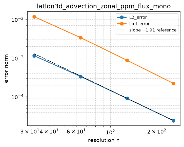
ppm_flux_D_lon_periodic
Source: grids/latlon3d/rules/ppm_flux_D_lon_periodic.esm
Rewrites ∂(U·q)/∂lon at priority 10 — match pattern:
{"op": "D", "args": [{"op": "*", "args": ["U", "q"]}], "wrt": "lon"}
where): fires only when U is a bare field shaped [lon_nodes, lat, lev]. Under import-edge renaming (§9.7.7) the wrt literal and this shape follow the renamed axis together, so the rule can be imported more than once (each instance scoped to its own grid) without a first-declared-wins collision. A consumer differentiating a compound inline expression must bind it to a declared shaped observed first.Discretization — one makearray tiling the output axes; boundary conditions live in the face regions of this same rule (esm-spec §9.6.8; later regions overwrite earlier, §4.3.2):
| Region | Treatment | Value |
|---|---|---|
lon ∈ [3, NLON−2], lat ∈ [1, NLAT], lev ∈ [1, NLEV] | interior | ppmflux_D_lon_unlim_interior(q, U)[i,j,k] = (dphi_lat[j] / ((dlon_deg·(3.14159265359 / 180))·dS_lat[j]))·(ppm_lev_flux(q[i−1, j, k], q[i, j, k], q[i+1, j, k], q[i+2, j, k], dlon_deg, dlon_deg, dlon_deg, dlon_deg, U[i+1, j, k]) − ppm_lev_flux(q[i−2, j, k], q[i−1, j, k], q[i, j, k], q[i+1, j, k], dlon_deg, dlon_deg, dlon_deg, dlon_deg, U[i, j, k])) for i ∈ [3, NLON−2], j ∈ lat, k ∈ lev |
lon = 1, lat ∈ [1, NLAT], lev ∈ [1, NLEV] | boundary face | ppmflux_D_lon_unlim_wrap_i1(q, U)[i,j,k] = (dphi_lat[j] / ((dlon_deg·(3.14159265359 / 180))·dS_lat[j]))·(ppm_lev_flux(q[NLON, j, k], q[1, j, k], q[2, j, k], q[3, j, k], dlon_deg, dlon_deg, dlon_deg, dlon_deg, U[2, j, k]) − ppm_lev_flux(q[NLON−1, j, k], q[NLON, j, k], q[1, j, k], q[2, j, k], dlon_deg, dlon_deg, dlon_deg, dlon_deg, U[1, j, k])) for i ∈ [1, 1], j ∈ lat, k ∈ lev |
lon = 2, lat ∈ [1, NLAT], lev ∈ [1, NLEV] | boundary face | ppmflux_D_lon_unlim_wrap_i2(q, U)[i,j,k] = (dphi_lat[j] / ((dlon_deg·(3.14159265359 / 180))·dS_lat[j]))·(ppm_lev_flux(q[1, j, k], q[2, j, k], q[3, j, k], q[4, j, k], dlon_deg, dlon_deg, dlon_deg, dlon_deg, U[3, j, k]) − ppm_lev_flux(q[NLON, j, k], q[1, j, k], q[2, j, k], q[3, j, k], dlon_deg, dlon_deg, dlon_deg, dlon_deg, U[2, j, k])) for i ∈ [2, 2], j ∈ lat, k ∈ lev |
lon = NLON−1, lat ∈ [1, NLAT], lev ∈ [1, NLEV] | boundary face | ppmflux_D_lon_unlim_wrap_iNm1(q, U)[i,j,k] = (dphi_lat[j] / ((dlon_deg·(3.14159265359 / 180))·dS_lat[j]))·(ppm_lev_flux(q[NLON−2, j, k], q[NLON−1, j, k], q[NLON, j, k], q[1, j, k], dlon_deg, dlon_deg, dlon_deg, dlon_deg, U[NLON, j, k]) − ppm_lev_flux(q[NLON−3, j, k], q[NLON−2, j, k], q[NLON−1, j, k], q[NLON, j, k], dlon_deg, dlon_deg, dlon_deg, dlon_deg, U[NLON−1, j, k])) for i ∈ [NLON−1, NLON−1], j ∈ lat, k ∈ lev |
lon = NLON, lat ∈ [1, NLAT], lev ∈ [1, NLEV] | boundary face | ppmflux_D_lon_unlim_wrap_iN(q, U)[i,j,k] = (dphi_lat[j] / ((dlon_deg·(3.14159265359 / 180))·dS_lat[j]))·(ppm_lev_flux(q[NLON−1, j, k], q[NLON, j, k], q[1, j, k], q[2, j, k], dlon_deg, dlon_deg, dlon_deg, dlon_deg, U[1, j, k]) − ppm_lev_flux(q[NLON−2, j, k], q[NLON−1, j, k], q[NLON, j, k], q[1, j, k], dlon_deg, dlon_deg, dlon_deg, dlon_deg, U[NLON, j, k])) for i ∈ [NLON, NLON], j ∈ lat, k ∈ lev |
UNLIMITED (centred) CW84 conservative flux-form ZONAL advection D(Uq, wrt: lon) on the latlon3d grid, with the eastward wind as a MATCHED OPERAND and the PERIODIC WRAP ENFORCED INSIDE THE RULE. A consuming model writes du/dt = -D(Uu, wrt: lon) + … and this rule lowers the whole compound. The exact zonal analogue of rules/ppm_flux_D_lev_noflux_bc, and the ACCURACY CEILING of the zonal family: the high-order, non-dissipative reference against which the monotone sibling rules/ppm_flux_D_lon_mono_periodic is measured.
THIS OPERATOR IS NOT UPWIND-BIASED, AND CANNOT BE. Its face value is the SHARED CW84 eq-(1.6) interface interpolant (../stencils/ppm_lev_flux, F = U * q_{i-1/2}, reused by import – its body is pure scalar algebra and knows nothing of lev), which does not depend on the sign of U at all. That is not an oversight: for the UNLIMITED reconstruction the parabola of the cell west of a face and the parabola of the cell east of it agree EXACTLY at the face they share, so the two one-sided donor values are identical and an ‘unlimited upwind PPM’ collapses, term for term, onto this centred flux. Upwind bias acquires content only once the eq (1.10) limiter has pulled the two cells’ endpoints apart, which is what the monotone sibling does.
WHAT THAT BUYS AND WHAT IT COSTS. Being centred, the flux-difference reduces algebraically to a 4th-order zonal derivative on the uniform lon mesh: MEASURED on the manufactured solution of problems/latlon3d_advection_zonal_ppm_flux (NLON = 32/64/128/256, NLAT and NLEV pinned; median pairwise rate) L2 3.99 and Linf 3.99 – clean fourth order, against the 1.88 / 1.94 the monotone sibling measures on the IDENTICAL MMS. (The last Linf rung softens to 2.5 because at NLON = 256 the truncation error, 3e-8, is approaching the integrator’s own floor at reltol 1e-11; the MEDIAN pairwise rate the gate uses is robust to it.) Verified numerically: against an independently hand-coded CW84 chain the lowered operator agrees to 0.0e+00 (bitwise); zonal conservation with the sign-reversing wind gives max |sum_i D| = 1.2e-14, 6.9e-17 relative; at q == 1 the face value collapses to 1.0 EXACTLY, so the tendency is BITWISE IDENTICAL to the donor-cell rule’s and to the pure mass divergence -weight*(U[i+1] - U[i]); and cyclic-shift equivariance, which pins the four wrap columns, holds to 0.0. The cost is boundedness: with no limiter this operator OVERSHOOTS at a sharp zonal gradient and can drive a chemical tracer NEGATIVE, and clipping the result to zero would silently destroy the exact mass conservation the flux form exists to provide. It is also not dissipative, so it does not damp the grid-scale noise a reversing wind excites. Use it to MEASURE (order studies, smooth manufactured solutions, and as the ceiling that localises the monotone sibling’s shortfall to its limiter); use the monotone sibling to RUN.
SUPPORT: FIVE CELLS, FOUR WRAP COLUMNS. A shared face value needs no per-cell endpoints, so the face reaches over four cells and the divergence over five (i-2..i+2): the interior is [3, NLON-2] and there are four wrap columns – two fewer cells and two fewer columns than the monotone sibling. Requires NLON >= 5 for a non-empty interior.
COMPOSITIONAL BODY: a makearray tiling [lon, lat, lev] with FIVE regions – the interior [3, NLON-2] uses ../stencils/ppmflux_D_lon_unlim_interior; the west columns i = 1,2 and the east columns i = NLON-1, NLON use ../stencils/ppmflux_D_lon_unlim_wrap_i{1,2,Nm1,N}. Every region is a full-rank slab aggregate (output_idx [i, j, k]).
THE METRIC IS THE DONOR RULE’S, UNCHANGED. In index form D(U*q, lon)[i,j,k] = ( dphi_lat[j] / (dlam dS_lat[j]) ) ( F_{i+1} - F_i ) with dlam = dlon_deg pi/180: the discrete spherical zonal flux divergence (1/(a cos phi)) d/dlam (U q). The two free names dphi_lat (shape [lat], the cell’s angular width in radians – latcell_dphi applied to the consumer’s phie, a HALF width at the caps) and dS_lat (shape [lat], the EXACT spherical cell-area weight sin(phie[j+1]) - sin(phie[j]) – latcell_area applied to the same phie), plus the inherited dlon_deg, are read from the consuming model’s scope: the same free-name contract by which the vertical rules read dz. NOTE WHAT IS ABSENT: no cos(phi) face-length factor, because on the zonal axis the cos(phi) of the metric and the cos(phi) of the zonal face length are the same number and cancel identically. The meridional rule needs coslat_e; this one does not. THIS RULE REPLACES ONLY THE FACE VALUE of rules/upwind1_flux_D_lon_periodic – a limited/interpolated parabola in place of the donor cell mean – and changes nothing else.
THE CELL WIDTHS ARE ALL ONE NUMBER, AND THAT IS EXACT, NOT AN APPROXIMATION. The lon axis is UNIFORM: at fixed j every cell in the row has the same physical width a cos(phi_j) dlam. The CW84 reconstruction is built from RATIOS of the widths and is degree-0 homogeneous in them, so scaling all of them by any positive constant leaves the face value bit-unchanged; the six width slots of the face-flux atom are therefore all fed the single scalar free name dlon_deg and the chain reduces to the exact uniform-mesh PPM. What matters is that they are IDENTICAL, which one name mentioned six times guarantees. (The VERTICAL siblings must pass six genuinely different dz[k] because the stretched vertical is non-uniform; that is the only structural difference between this family and theirs.)
THE PERIODIC WRAP IS ENFORCED BY THE RULE, SO CONSERVATION CANNOT BE BROKEN FROM OUTSIDE – AND ON A PERIODIC AXIS THE BOUNDARY COLUMNS DROP NOTHING. They are not truncated one-sided stencils; they are FULL-SUPPORT PPM columns with ROTATED indices (cell 1’s i-1 is NLON, its i-2 is NLON-1, its i-3 is NLON-2). Cell NLON’s EAST face and cell 1’s WEST face are THE SAME FACE of the closed circle, and the two wrap stencils build it from the SAME cells, the SAME widths and the SAME face velocity U[1] in the SAME argument order, so the two expressions lower to the same AST and evaluate to the SAME DOUBLE. sum_i (F_{i+1} - F_i) therefore telescopes to EXACTLY 0.0 in IEEE arithmetic, for ANY q and ANY U – including a deliberately non-periodic one. ELEMENT U[NLON+1,j,k] IS NEVER READ (the east face of cell NLON reuses U[1]); whatever a consumer stores there is ignored. The lon_nodes axis is sized NLON+1 all the same, so a future REGIONAL (non-periodic) zonal rule has a genuine east boundary face to close against. This is the periodic-axis counterpart of the discipline by which the vertical no-flux rules STRUCTURALLY OMIT the wall flux rather than forming it and multiplying by zero.
COMPOUND MATCH, AND WHY IT CANNOT COLLIDE. The match is D(Uq, wrt: lon) at priority 10, so under the esm-spec 9.6.3 outermost-first compound precedence it fires on the whole product before any plain-D lon rule (upwind1_D_lon_periodic, ppm_D_lon_periodic) can lower an inner derivative. Matching is STRUCTURAL and NON-COMMUTATIVE: the wind MUST be written on the LEFT of the product. A model that also carries zonal diffusion contains D(khD(u, wrt: lon), wrt: lon), whose outer node is ALSO a D of a two-factor product; it is the esm-spec 9.6.1 where SHAPE CONSTRAINT, not priority, that separates them, because a shape constraint is satisfied only by a BARE VARIABLE-REFERENCE STRING and the diffusion term’s inner factor is a compound D node. Advection and diffusion therefore compose in one equation, each firing on its own term.
ACCURACY SIBLINGS OVER ONE CONTRACT, SELECTED BY IMPORT. This rule matches the SAME compound D(Uq, wrt: lon) at the SAME priority 10 as rules/upwind1_flux_D_lon_periodic (first-order donor cell) and as the other member of this PPM pair. That is deliberate and is the established pattern on this grid (the vertical ppm_flux_D_lev_ pair does exactly the same): a consuming PROBLEM imports EXACTLY ONE of them, and there is no priority game to arbitrate between them and none is wanted.
Semi-discrete (method-of-lines): the ODE integrator owns dt, so this is NOT the fully-discrete flux-form semi-Lagrangian TPCORE scheme of Lin & Rood (1996) that GEOS-Chem runs operationally (see the SCHEME CAVEAT in grids/latlon3d/grid.esm). The zonal circle must actually close (NLON dlon_deg = 360); on a regional mesh this rule is a modeling error.
References
- Colella, P., & Woodward, P. R. (1984). The Piecewise Parabolic Method (PPM) for gas-dynamical simulations. Journal of Computational Physics, 54(1), 174-201.
doi:10.1016/0021-9991(84)90143-8 - Lin, S.-J., & Rood, R. B. (1996). Multidimensional flux-form semi-Lagrangian transport schemes. Monthly Weather Review, 124(9), 2046-2070.
doi:10.1175/1520-0493(1996)124<2046:MFFSLT>2.0.CO;2 - Colella, P., & Sekora, M. D. (2008). A limiter for PPM that preserves accuracy at smooth extrema. Journal of Computational Physics, 227(15), 7069-7076.
doi:10.1016/j.jcp.2008.03.034 - Williamson, D. L., Drake, J. B., Hack, J. J., Jakob, R., & Swarztrauber, P. N. (1992). A standard test set for numerical approximations to the shallow water equations in spherical geometry. Journal of Computational Physics, 102(1), 211-224. (Spherical lat-lon metric factors for the zonal flux divergence.)
doi:10.1016/S0021-9991(05)80016-6 - LeVeque, R. J. (2002). Finite Volume Methods for Hyperbolic Problems. Cambridge University Press. Section 4.1 (the donor-cell upwind flux; the upwind selection is the same whatever sub-grid reconstruction supplies the two one-sided face values).
Conformance fixtures
- ast:
latlon3d_ppm_flux_D_lon_periodic— statusactive - convergence:
latlon3d_advection_zonal_ppm_flux— statusactive
Convergence — case latlon3d_advection_zonal_ppm_flux
Error norms read from the committed golden tests/conformance/convergence/latlon3d_advection_zonal_ppm_flux/golden/errors.json (binding: julia; nothing recomputed for display).
| n | L2_error | observed order | Linf_error | observed order |
|---|---|---|---|---|
| 32 | 6.731e-06 | — | 4.195e-05 | — |
| 64 | 4.241e-07 | 3.99 | 2.648e-06 | 3.99 |
| 128 | 2.656e-08 | 4.00 | 1.656e-07 | 4.00 |
Expected order: 4 (± 0.15).
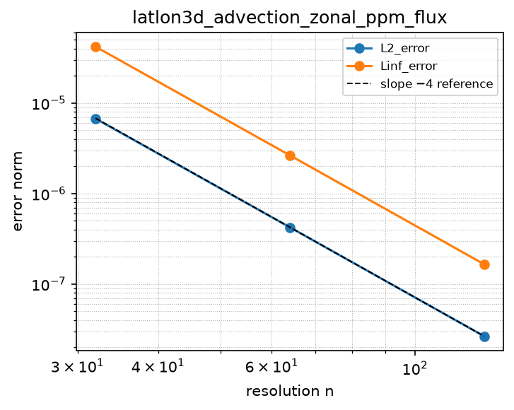
upwind1_D_lon_periodic
Source: grids/latlon3d/rules/upwind1_D_lon_periodic.esm
Rewrites ∂f/∂lon — match pattern:
{"op": "D", "args": ["f"], "wrt": "lon"}
where): fires only when f is a bare field shaped [lon, lat, lev]. Under import-edge renaming (§9.7.7) the wrt literal and this shape follow the renamed axis together, so the rule can be imported more than once (each instance scoped to its own grid) without a first-declared-wins collision. A consumer differentiating a compound inline expression must bind it to a declared shaped observed first.Discretization — one makearray tiling the output axes; boundary conditions live in the face regions of this same rule (esm-spec §9.6.8; later regions overwrite earlier, §4.3.2):
| Region | Treatment | Value |
|---|---|---|
lon ∈ [2, NLON], lat ∈ [1, NLAT], lev ∈ [1, NLEV] | interior | upwind1_D_lon_interior(f)[i,j,k] = (f[i, j, k] − f[i−1, j, k]) / dlon_deg for i ∈ [2, NLON], j ∈ lat, k ∈ lev |
lon = 1, lat ∈ [1, NLAT], lev ∈ [1, NLEV] | boundary face | upwind1_D_lon_wrap_face(f)[i,j,k] = (f[1, j, k] − f[NLON, j, k]) / dlon_deg for i ∈ [1, 1], j ∈ lat, k ∈ lev |
First-order upwind (backward) first derivative along longitude with periodic (wrap) boundary on the latlon3d grid — the rank-3 (lon x lat x lev) extension of grids/latlon/rules/upwind1_D_lon_periodic, for zonal advection with non-negative angular velocity (flow toward increasing longitude) in a 3-D tracer-transport model such as GEOS-Chem Classic. Matches D(f, wrt: lon), a PER-DEGREE derivative. The body is a makearray tiling [lon, lat, lev] with exactly two regions, each filled by a thin apply of a factored stencil: interior columns [2, NLON] x lat x lev use ../stencils/upwind1_D_lon_interior; the single i=1 face column uses ../stencils/upwind1_D_lon_wrap_face, which wraps to (f[1] - f[NLON]) / dlon_deg. Only one face column is special (upwind needs an upstream neighbor toward smaller lon, which every column but i=1 has), so the tiling is interior + one wrap face on the lon axis, spanning the full lat and lev extents. Both regions are full-rank slab aggregates (output_idx [i, j, k]) so every binding’s simulator fills the (1 x NLAT x NLEV) wrap slab without rank promotion. The scheme is O(dlon_deg) at every column and conserves sum(f) exactly (the periodic wrap telescopes). dlon_deg is the inherited consumer-supplied zonal spacing free name (grids/latlon3d/grid.esm); the rule never assumes the global extent, but composing it with a non-closing regional grid is a modeling error. Match scoping: wrt: lon plus where: {f: {shape: [lon, lat, lev]}} (esm-spec 9.6.1) at DEFAULT priority, so it fires only on the longitudinal derivative of a bare field declared over THIS grid’s lon x lat x lev index sets — not on a 2-D latlon field (shape [lon, lat]) and not on any unrelated D(., wrt: lon) — and, under import-edge renaming (esm-spec 9.7.7), the wrt literal and the where shape follow the renamed axis together, so two latlon3d instances coexist scoped to their own meshes. The constraint requires a bare shaped variable; a consumer differentiating a compound inline expression must bind it to a declared lon x lat x lev observed first. Sign convention: upwind for flow toward +lon; a westward variant belongs in a separate rule.
References
- LeVeque, R. J. (2002). Finite Volume Methods for Hyperbolic Problems. Cambridge University Press. Section 4.8 (upwind methods on periodic domains).
Conformance fixtures
- ast:
latlon3d_upwind1_D_lon_periodic— statusactive - ast:
upwind1_D_lon_periodic— statusactive - convergence:
latlon3d_advection_zonal_upwind— statusactive - simulation:
latlon3d_advection_3d— statusactive
Convergence — case latlon3d_advection_zonal_upwind
Error norms read from the committed golden tests/conformance/convergence/latlon3d_advection_zonal_upwind/golden/errors.json (binding: julia; nothing recomputed for display).
| n | L2_error | observed order | Linf_error | observed order |
|---|---|---|---|---|
| 16 | 1.424e-01 | — | 1.420e-01 | — |
| 32 | 7.414e-02 | 0.94 | 7.409e-02 | 0.94 |
| 64 | 3.781e-02 | 0.97 | 3.780e-02 | 0.97 |
| 128 | 1.909e-02 | 0.99 | 1.909e-02 | 0.99 |
Expected order: 1 (± 0.15).
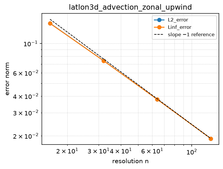
upwind1_flux_D_lat_polar
Source: grids/latlon3d/rules/upwind1_flux_D_lat_polar.esm
Rewrites ∂(V·q)/∂lat at priority 10 — match pattern:
{"op": "D", "args": [{"op": "*", "args": ["V", "q"]}], "wrt": "lat"}
where): fires only when q is a bare field shaped [lon, lat, lev]; V is a bare field shaped [lon, lat_nodes, lev]. Under import-edge renaming (§9.7.7) the wrt literal and this shape follow the renamed axis together, so the rule can be imported more than once (each instance scoped to its own grid) without a first-declared-wins collision. A consumer differentiating a compound inline expression must bind it to a declared shaped observed first.Discretization — one makearray tiling the output axes; boundary conditions live in the face regions of this same rule (esm-spec §9.6.8; later regions overwrite earlier, §4.3.2):
| Region | Treatment | Value |
|---|---|---|
lon ∈ [1, NLON], lat ∈ [2, NLAT−1], lev ∈ [1, NLEV] | interior | upwind1_D_lat_flux_interior(q, V)[i,j,k] = (upwind_lev_face_flux(q[i, j, k], q[i, j+1, k], V[i, j+1, k])·coslat_e[j+1] − upwind_lev_face_flux(q[i, j−1, k], q[i, j, k], V[i, j, k])·coslat_e[j]) / dS_lat[j] for i ∈ lon, j ∈ [2, NLAT−1], k ∈ lev |
lon ∈ [1, NLON], lat = 1, lev ∈ [1, NLEV] | boundary face | upwind1_D_lat_flux_cap_s(q, V)[i,j,k] = (upwind_lev_face_flux(q[i, 1, k], q[i, 2, k], V[i, 2, k])·coslat_e[2]) / dS_lat[1] for i ∈ lon, j ∈ [1, 1], k ∈ lev |
lon ∈ [1, NLON], lat = NLAT, lev ∈ [1, NLEV] | boundary face | upwind1_D_lat_flux_cap_n(q, V)[i,j,k] = (−(upwind_lev_face_flux(q[i, NLAT−1, k], q[i, NLAT, k], V[i, NLAT, k])·coslat_e[NLAT])) / dS_lat[NLAT] for i ∈ lon, j ∈ [NLAT, NLAT], k ∈ lev |
Conservative FLUX-FORM first-order-upwind MERIDIONAL advection D(Vq, wrt: lat) on the latlon3d grid, with the pole treated as a ZERO-LENGTH FACE (no-flux) at both ends. The consuming model writes du/dt = -D(Vu, wrt: lat) + … and this rule lowers the whole compound; V is the face-staggered northward wind, INSIDE the operator, exactly as W is in the vertical sibling upwind1_flux_D_lev_noflux_bc.
WHAT THE OPERATOR IS. In index form D[i,j,k] = ( F_{j+1} coslat_e[j+1] - F_j coslat_e[j] ) / dS_lat[j], the discrete form of the spherical meridional flux divergence (1/(a cos phi)) d/dphi ( cos(phi) v q ). F_j is the donor-cell flux at face j (the SOUTHERN edge of cell j) computed by the axis-neutral atom upwind_lev_face_flux, coslat_e is the face-LENGTH weight cos(phi_e) and dS_lat the EXACT spherical cell-AREA weight sin(phi_e[j+1]) - sin(phi_e[j]). Both are read as FREE NAMES from the consuming model’s scope – the same contract by which the vertical rules read dz – and the consumer builds them from the grid templates: an observed phie = lat_edge() of shape [lat_nodes], then coslat_e = coslat_edge(phie) and dS_lat = latcell_area(phie). Because the divergence differences FACE fluxes and the two pole-wall terms are omitted outright, the fluxes telescope and sum_j dS_lat[j] D[i,j,k] is zero to machine precision for ANY q and V: meridional transport conserves tracer mass exactly.
WHY lat_nodes IS THE DISCRIMINATOR. The match is the compound D(Vq, wrt: lat) at priority 10, so under the esm-spec 9.6.3 outermost-first precedence it fires on the whole product before any plain-D lat rule (central_D_lat_, upwind1_D_lat_) can lower an inner derivative. Matching is STRUCTURAL and NON-COMMUTATIVE, so the wind MUST be written on the LEFT of the product. A model that also carries meridional diffusion contains D(khD(u, wrt: lat), wrt: lat), whose outer node is ALSO a D of a two-factor product; it is the esm-spec 9.6.1 where SHAPE CONSTRAINT, not priority, that separates them, because a shape constraint is satisfied only by a BARE VARIABLE-REFERENCE STRING and the diffusion term’s inner factor is a compound D node. The constraint on V additionally requires the index-set NAME list [lon, lat_nodes, lev]: a cell-centred [lon, lat, lev] field can never be mistaken for a face wind even at sizes where NLAT+1 collides with another axis.
ACCURACY AT THE POLES – READ THIS BEFORE TRUSTING A POINTWISE ERROR NORM. The half-polar cap divides an O(dphi) donor-cell face-reconstruction error by an O(dphi^2) cell area, and more generally row j divides by a cell area of O(cos(phi_j) dphi), so the truncation error of this operator scales as O(dphi / cos(phi)). The consequences are precise and were MEASURED on the full 2-D operator (rotated solid-body rotation crossed with a 2-D smooth tracer; (NLON,NLAT) = (32,17)/(64,33)/(128,65)/(256,129); pairwise orders): (1) at any FIXED latitude the scheme converges at first order – Linf restricted to |lat| < 60 gives orders 1.01/1.00/1.00, and to |lat| < 80 gives 0.89/1.04/1.01. (2) Linf over the WHOLE SPHERE does NOT converge – orders 0.47/0.24/0.12, decaying toward zero. This is not a defect of the scheme: the row nearest the pole always sits at cos(phi) ~ dphi, so its error is O(dphi/dphi) = O(1) at EVERY resolution. It is the lat-lon coordinate singularity. (3) the AREA (mass) WEIGHT is O(cos(phi)) and cancels the 1/cos(phi) EXACTLY: the mass-weighted error converges at first order – Linf of (error * cos(phi)) gives orders 1.02/1.01/1.01, and area-weighted L1/L2 give 1.00/1.00/1.00 and 0.97/0.98/0.98. Since this operator’s contract is CONSERVATION of tracer mass, the mass-weighted norm is the meaningful one, and in it the scheme is cleanly first order. TWO FIXES THAT DO NOT WORK, both measured, so that neither is re-attempted: raising the reconstruction order does NOT restore pointwise polar convergence (a 2nd-order centred reconstruction on BOTH axes still decays: 0.72/0.53/0.34), and neither does a TRUE POLAR CAP (merging each polar row into one spherical cap cell and driving it by the net ring influx). The true polar cap does fix the cap ROW cleanly – its order goes from 0 to 0.99/1.00/1.00, because at the pole both V and dq/dphi are pure first harmonics in lambda and the zonal mean of their product vanishes identically – but rows 2, 3, … still carry O(dphi/cos(phi)) and Linf still stalls at 0.47/0.24/0.12. Nothing local to the spatial operator fixes this; the operational remedy is a POLAR FILTER applied at runtime, outside the method-of-lines operator. A COMMON MISREADING TO AVOID: it is tempting to argue that fields smooth on the sphere are safe because a smooth vector field has V -> 0 at the poles and a smooth scalar has dq/dphi -> 0 there. BOTH premises are false for genuinely 2-D fields, and only hold for LATITUDE-ONLY ones. q = cos(phi)cos(lambda) is merely the Cartesian x-coordinate – perfectly smooth – yet its pole derivative is -cos(lambda) != 0; and rotated solid-body rotation, the canonical smooth flow on a sphere, has v = -u0 sin(lambda) sin(alpha), which does not vanish at the poles either. The spherical-component basis is singular at the pole even where the vector field is not. WHAT HOLDS FOR ANY WIND, with no smoothness precondition at all: the scheme is EXACTLY conservative (the interior fluxes telescope and the pole-face terms are structurally absent, so sum_j D[j] * dS_lat[j] = 0 to machine precision – measured 2e-17 relative), and it is BIT-EXACTLY free-stream-preserving (at q == 1 the donor flux collapses to F = 0.5*(V*(1+1) - |V|*(1-1)) = V with every IEEE operation exact, so a constant tracer stays constant to the last bit). Those two properties, not the pointwise order, are what a conservative tracer-transport scheme owes its caller. ACCURACY AND SCOPE. Donor-cell upwinding is O(dphi) and unconditionally monotone: no new extrema, no negative concentrations. It is the first rung; an upwind-biased PPM reconstruction refines it by replacing the donor cell value with a parabola endpoint, reusing this same face-flux and divergence structure. Semi-discrete (method-of-lines), so it is NOT the fully-discrete flux-form semi-Lagrangian TPCORE scheme of Lin & Rood (1996) that GEOS-Chem runs operationally (see the SCHEME CAVEAT in grids/latlon3d/grid.esm). Requires NLAT >= 3.
References
- LeVeque, R. J. (2002). Finite Volume Methods for Hyperbolic Problems. Cambridge University Press. Section 4.1 (the upwind / donor-cell flux and its branch-free algebraic form F = 1/2[u(qL+qR) - |u|(qR-qL)]).
- Lin, S.-J., & Rood, R. B. (1996). Multidimensional flux-form semi-Lagrangian transport schemes. Monthly Weather Review, 124(9), 2046-2070.
doi:10.1175/1520-0493(1996)124<2046:MFFSLT>2.0.CO;2 - Jacobson, M. Z. (2005). Fundamentals of Atmospheric Modeling (2nd ed.). Cambridge University Press. Chapter 6 (finite-volume flux-form tracer transport; consistency with continuity).
Conformance fixtures
- ast:
latlon3d_upwind1_flux_D_lat_polar— statusactive - convergence:
latlon3d_advection_meridional_upwind_flux— statusactive - simulation:
latlon3d_transport_cwc_3d— statusactive
Convergence — case latlon3d_advection_meridional_upwind_flux
Error norms read from the committed golden tests/conformance/convergence/latlon3d_advection_meridional_upwind_flux/golden/errors.json (binding: julia; nothing recomputed for display).
| n | L2_error | observed order | Linf_error | observed order |
|---|---|---|---|---|
| 16 | 3.823e-03 | — | 1.979e-02 | — |
| 32 | 1.941e-03 | 0.98 | 9.978e-03 | 0.99 |
| 64 | 9.793e-04 | 0.99 | 4.972e-03 | 1.01 |
| 128 | 4.919e-04 | 0.99 | 2.483e-03 | 1.00 |
Expected order: 1 (± 0.15).
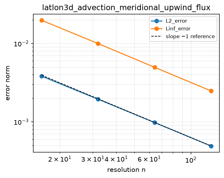
upwind1_flux_D_lev_noflux_bc
Source: grids/latlon3d/rules/upwind1_flux_D_lev_noflux_bc.esm
Rewrites ∂(W·q)/∂lev at priority 10 — match pattern:
{"op": "D", "args": [{"op": "*", "args": ["W", "q"]}], "wrt": "lev"}
where): fires only when q is a bare field shaped [lon, lat, lev]; W is a bare field shaped [lon, lat, lev_nodes]. Under import-edge renaming (§9.7.7) the wrt literal and this shape follow the renamed axis together, so the rule can be imported more than once (each instance scoped to its own grid) without a first-declared-wins collision. A consumer differentiating a compound inline expression must bind it to a declared shaped observed first.Discretization — one makearray tiling the output axes; boundary conditions live in the face regions of this same rule (esm-spec §9.6.8; later regions overwrite earlier, §4.3.2):
| Region | Treatment | Value |
|---|---|---|
lon ∈ [1, NLON], lat ∈ [1, NLAT], lev ∈ [2, NLEV−1] | interior | upwind1_D_lev_flux_interior(q, W)[i,j,k] = (upwind_lev_face_flux(q[i, j, k], q[i, j, k+1], W[i, j, k+1]) − upwind_lev_face_flux(q[i, j, k−1], q[i, j, k], W[i, j, k])) / dz[k] for i ∈ lon, j ∈ lat, k ∈ [2, NLEV−1] |
lon ∈ [1, NLON], lat ∈ [1, NLAT], lev = 1 | boundary face | upwind1_D_lev_flux_nf_k1(q, W)[i,j,k] = upwind_lev_face_flux(q[i, j, 1], q[i, j, 2], W[i, j, 2]) / dz[1] for i ∈ lon, j ∈ lat, k ∈ [1, 1] |
lon ∈ [1, NLON], lat ∈ [1, NLAT], lev = NLEV | boundary face | upwind1_D_lev_flux_nf_kN(q, W)[i,j,k] = (−upwind_lev_face_flux(q[i, j, NLEV−1], q[i, j, NLEV], W[i, j, NLEV])) / dz[NLEV] for i ∈ lon, j ∈ lat, k ∈ [NLEV, NLEV] |
Conservative FLUX-FORM first-order-upwind vertical advection d/dz(w q) on the latlon3d non-uniform vertical, with rigid NO-FLUX walls at both the surface and the model top. The consuming model writes its transport equation as du/dt = -D(W*u, wrt: lev) + … and this rule lowers the whole compound.
THE VELOCITY IS INSIDE THE OPERATOR. This is the substantive difference from the pre-existing advective-form operators on this grid (upwind1_D_lon_periodic, central_D_lev_zero_grad_bc, the ppm_D_* family), which match a BARE derivative D(q, wrt: axis) and require the consuming model to multiply by a velocity from OUTSIDE. That is only correct for a CONSTANT velocity, for which w dq/dz and d(wq)/dz coincide; it silently ceases to conserve tracer mass the moment the velocity varies in space, which every real wind field does. Matching the compound D(Wq) instead lets the operator (a) accept a genuine three-dimensional face-staggered velocity field, (b) difference the flux wq at faces so that mass telescopes exactly, and (c) SEE THE SIGN of the local face velocity, which is what makes upwinding possible at all for a wind that reverses – the pre-existing operators hard-code a single flow direction.
COMPOUND MATCH, AND WHY IT CANNOT COLLIDE WITH THE DIFFUSION RULE. The match pattern is D(Wq, wrt: lev) at priority 10, so under the esm-spec 9.6.3 outermost-first compound precedence it fires on the whole product before any plain-D rule can lower an inner derivative. Matching is STRUCTURAL and NON-COMMUTATIVE, so the velocity MUST be written on the LEFT of the product. A model that also carries vertical diffusion contains the term D(kzD(u, wrt: lev), wrt: lev), whose outer node is ALSO a D of a two-factor product – so this rule’s pattern structurally matches it too, binding W := kz and q := D(u, wrt: lev). It is the where constraint, NOT priority, that separates them: by esm-spec 9.6.1 a shape constraint is satisfied only when the bound sub-AST is a BARE VARIABLE-REFERENCE STRING, and a compound sub-AST fails it. The diffusion term binds q to the compound D(u, wrt: lev), so the constraint on q fails and this rule is filtered out at that node BEFORE the priority/declaration-order selection ever runs. The separation is therefore a structural guarantee of the shape-constraint semantics rather than a priority race, and it holds in both directions – the diffusion rule’s pattern requires its inner factor to be structurally a D node, which a bare tracer q is not. Advection and diffusion consequently compose in a single equation, each firing on its own term.
SHAPES. The tracer q is declared over [lon, lat, lev] (cell centres) and the velocity W over [lon, lat, lev_nodes] (the NLEV+1 face axis), positive UPWARD. Face k is the lower edge of cell k; face 1 is the ground and face NLEV+1 the model top, and the velocities stored in those two faces are never read because the wall fluxes are literally absent.
ACCURACY AND SCOPE. Donor-cell upwinding is O(dz) and unconditionally monotone: it will not manufacture new extrema or negative concentrations, which is the property that matters most for a chemical tracer. It is deliberately the FIRST rung – the upwind-biased PPM reconstruction refines it by replacing the donor cell value with a parabola endpoint, reusing this same face-flux and divergence structure. Note that a semi-discrete (method-of-lines) flux-form scheme is NOT the fully-discrete flux-form semi-Lagrangian TPCORE scheme of Lin & Rood (1996) that GEOS-Chem runs operationally: TPCORE carries the Courant number inside the operator and cannot be expressed method-of-lines (see the SCHEME CAVEAT in grids/latlon3d/grid.esm). Requires NLEV >= 3.
References
- LeVeque, R. J. (2002). Finite Volume Methods for Hyperbolic Problems. Cambridge University Press. Section 4.1 (the upwind / donor-cell flux and its branch-free algebraic form F = 1/2[u(qL+qR) - |u|(qR-qL)]).
- Lin, S.-J., & Rood, R. B. (1996). Multidimensional flux-form semi-Lagrangian transport schemes. Monthly Weather Review, 124(9), 2046-2070.
doi:10.1175/1520-0493(1996)124<2046:MFFSLT>2.0.CO;2 - Jacobson, M. Z. (2005). Fundamentals of Atmospheric Modeling (2nd ed.). Cambridge University Press. Chapter 6 (finite-volume flux-form tracer transport; consistency with continuity).
Conformance fixtures
- ast:
latlon3d_upwind1_flux_D_lev_noflux_bc— statusactive - convergence:
latlon3d_advection_vertical_upwind_flux— statusactive - convergence:
latlon3d_transport_cwc_mms— statusactive - simulation:
latlon3d_transport_cwc_3d— statusactive
Convergence — case latlon3d_advection_vertical_upwind_flux
Error norms read from the committed golden tests/conformance/convergence/latlon3d_advection_vertical_upwind_flux/golden/errors.json (binding: julia; nothing recomputed for display).
| n | L2_error | observed order | Linf_error | observed order |
|---|---|---|---|---|
| 32 | 2.657e-02 | — | 6.537e-02 | — |
| 64 | 1.388e-02 | 0.94 | 3.804e-02 | 0.78 |
| 128 | 7.126e-03 | 0.96 | 2.028e-02 | 0.91 |
| 256 | 3.641e-03 | 0.97 | 1.020e-02 | 0.99 |
Expected order: 1 (± 0.15).
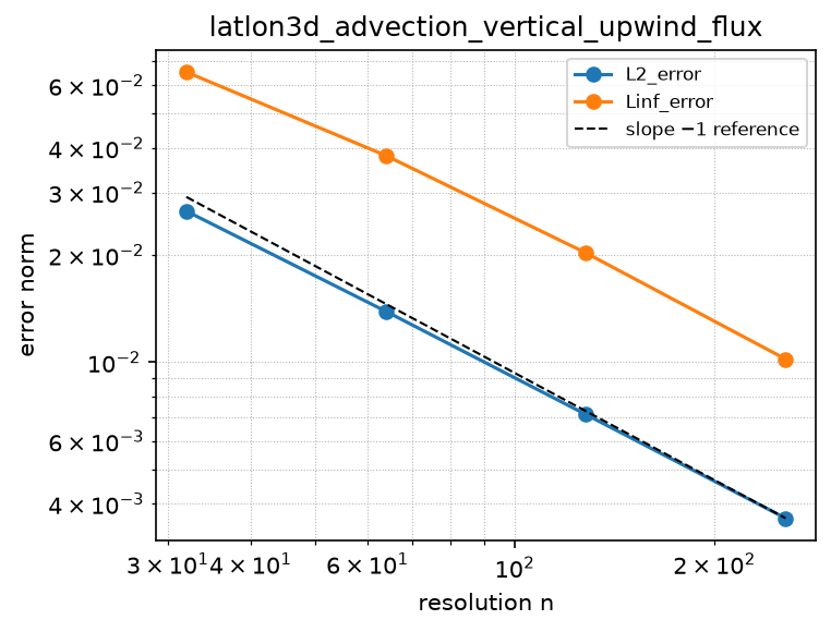
Convergence — case latlon3d_transport_cwc_mms
Error norms read from the committed golden tests/conformance/convergence/latlon3d_transport_cwc_mms/golden/errors.json (binding: julia; nothing recomputed for display).
| n | L2_error | observed order | Linf_error | observed order |
|---|---|---|---|---|
| 32 | 2.169e-03 | — | 1.694e-02 | — |
| 64 | 1.092e-03 | 0.99 | 9.106e-03 | 0.90 |
| 128 | 5.480e-04 | 1.00 | 4.715e-03 | 0.95 |
| 256 | 2.747e-04 | 1.00 | 2.399e-03 | 0.98 |
Expected order: 1 (± 0.15).
upwind1_flux_D_lon_periodic
Source: grids/latlon3d/rules/upwind1_flux_D_lon_periodic.esm
Rewrites ∂(U·q)/∂lon at priority 10 — match pattern:
{"op": "D", "args": [{"op": "*", "args": ["U", "q"]}], "wrt": "lon"}
where): fires only when q is a bare field shaped [lon, lat, lev]; U is a bare field shaped [lon_nodes, lat, lev]. Under import-edge renaming (§9.7.7) the wrt literal and this shape follow the renamed axis together, so the rule can be imported more than once (each instance scoped to its own grid) without a first-declared-wins collision. A consumer differentiating a compound inline expression must bind it to a declared shaped observed first.Discretization — one makearray tiling the output axes; boundary conditions live in the face regions of this same rule (esm-spec §9.6.8; later regions overwrite earlier, §4.3.2):
| Region | Treatment | Value |
|---|---|---|
lon ∈ [2, NLON−1], lat ∈ [1, NLAT], lev ∈ [1, NLEV] | interior | upwind1_D_lon_flux_interior(q, U)[i,j,k] = (dphi_lat[j] / ((dlon_deg·(3.14159265359 / 180))·dS_lat[j]))·(upwind_lev_face_flux(q[i, j, k], q[i+1, j, k], U[i+1, j, k]) − upwind_lev_face_flux(q[i−1, j, k], q[i, j, k], U[i, j, k])) for i ∈ [2, NLON−1], j ∈ lat, k ∈ lev |
lon = 1, lat ∈ [1, NLAT], lev ∈ [1, NLEV] | boundary face | upwind1_D_lon_flux_wrap_i1(q, U)[i,j,k] = (dphi_lat[j] / ((dlon_deg·(3.14159265359 / 180))·dS_lat[j]))·(upwind_lev_face_flux(q[1, j, k], q[2, j, k], U[2, j, k]) − upwind_lev_face_flux(q[NLON, j, k], q[1, j, k], U[1, j, k])) for i ∈ [1, 1], j ∈ lat, k ∈ lev |
lon = NLON, lat ∈ [1, NLAT], lev ∈ [1, NLEV] | boundary face | upwind1_D_lon_flux_wrap_iN(q, U)[i,j,k] = (dphi_lat[j] / ((dlon_deg·(3.14159265359 / 180))·dS_lat[j]))·(upwind_lev_face_flux(q[NLON, j, k], q[1, j, k], U[1, j, k]) − upwind_lev_face_flux(q[NLON−1, j, k], q[NLON, j, k], U[NLON, j, k])) for i ∈ [NLON, NLON], j ∈ lat, k ∈ lev |
Conservative FLUX-FORM first-order-upwind ZONAL advection D(Uq, wrt: lon) on the latlon3d grid, with the PERIODIC WRAP ENFORCED INSIDE THE RULE. The consuming model writes its transport equation as du/dt = -D(Uu, wrt: lon) + … and this rule lowers the whole compound; U is the face-staggered eastward wind, INSIDE the operator, exactly as W is in the vertical sibling upwind1_flux_D_lev_noflux_bc and V in the meridional sibling upwind1_flux_D_lat_polar.
WHAT THE OPERATOR IS. In index form D[i,j,k] = ( dphi_lat[j] / (dlam dS_lat[j]) ) ( F_{i+1} - F_i ) with dlam = dlon_deg pi/180, the discrete form of the spherical zonal flux divergence (1/(a cos(phi))) d/dlam (U q). F_i is the donor-cell flux through face i (the WESTERN edge of cell i), computed by the axis-neutral atom upwind_lev_face_flux from qL = q[i-1,j,k], qR = q[i,j,k] and w = U[i,j,k]. The metric weight reads TWO free names from the consuming model’s scope – dphi_lat (shape [lat], the cell’s angular width in radians, = the grid’s latcell_dphi applied to the consumer’s phie) and dS_lat (shape [lat], the EXACT spherical cell-area weight sin(phie[j+1]) - sin(phie[j]), = latcell_area applied to the same phie) – plus the inherited dlon_deg, the same free-name contract by which the vertical rules read dz. NOTE WHAT IS ABSENT: no cos(phi) face-length factor appears, because on the zonal axis the cos(phi) of the metric and the cos(phi) of the face length are the same number and cancel identically; the meridional rule needs coslat_e, this one does not.
THE WRAP IS ENFORCED BY THE RULE, WHICH IS WHY CONSERVATION CANNOT BE BROKEN FROM OUTSIDE. Three makearray regions tile the lon axis: the two wrap columns are not boundary conditions in the usual sense but the two halves of ONE SHARED FACE. Column 1 takes its west face as F_1 = donor(q[NLON], q[1], U[1]); column NLON takes its east face as F_{NLON+1} = donor(q[NLON], q[1], U[1]) – THE SAME q VALUES AND THE SAME WIND ELEMENT U[1], NOT U[NLON+1]. The two expressions are therefore BIT-IDENTICAL, so the boundary terms of the row sum sum_i (F_{i+1} - F_i) = F_{NLON+1} - F_1 cancel bit-for-bit and zonal mass is conserved for ANY q and ANY U – including a deliberately NON-PERIODIC U. (What is exact is the CANCELLATION: F_{NLON+1} and F_1 are the same double. The accumulated floating-point row sum of the individually-rounded per-cell divergences is then zero to machine precision – measured max |sum_i D| = 3.6e-15, 6.8e-17 relative – and it does not move by one bit when U[NLON+1] is poisoned.) ELEMENT U[NLON+1,j,k] IS CONSEQUENTLY NEVER READ: whatever a consumer stores in the last face of the zonal wind is ignored (measured: setting it to 1e6 changes not one bit of the output), the same discipline by which the vertical no-flux rules never read W at the wall faces and the polar rule never reads V at the pole faces. The lon_nodes axis is sized NLON+1 all the same, so a future REGIONAL (non-periodic) zonal rule has a genuine east boundary face to close against.
COMPOUND MATCH, AND WHY IT CANNOT COLLIDE. The match is D(Uq, wrt: lon) at priority 10, so under the esm-spec 9.6.3 outermost-first compound precedence it fires on the whole product before any plain-D lon rule (upwind1_D_lon_periodic, ppm_D_lon_periodic) can lower an inner derivative. Matching is STRUCTURAL and NON-COMMUTATIVE, so the wind MUST be written on the LEFT of the product. A model that also carries zonal diffusion contains D(khD(u, wrt: lon), wrt: lon), whose outer node is ALSO a D of a two-factor product; it is the esm-spec 9.6.1 where SHAPE CONSTRAINT, not priority, that separates them, because a shape constraint is satisfied only by a BARE VARIABLE-REFERENCE STRING and the diffusion term’s inner factor is a compound D node. The constraint on U additionally requires the index-set NAME list [lon_nodes, lat, lev]: a cell-centred [lon, lat, lev] field can never be mistaken for a face wind even at sizes where NLON+1 collides with another axis.
ACCURACY AND SCOPE. Donor-cell upwinding is O(dlam) and unconditionally monotone: no new extrema, no negative concentrations. MEASURED (forced-steady MMS, q*(lambda) = 2 + sin(lambda) initialised to its exact cell mean, a sign-CHANGING wind U = U0 (0.5 + cos(lambda)) a(j) b(k) so both donor branches fire, NLON = 32/64/128/256 with NLAT and NLEV pinned): pairwise orders L2 0.94 / 0.97 / 0.99 (median 0.97) and Linf 0.91 / 0.94 / 0.97 (median 0.94) – cleanly first order, approaching 1 from below as a donor-cell scheme does. The sweep refines ONLY the zonal axis, so the polar metric weights are exercised (the caps’ dphi_lat/dS_lat ratio is the largest in the mesh) but not refined, which keeps the lat-lon coordinate singularity – the thing that stalls the MERIDIONAL operator’s pointwise Linf, see upwind1_flux_D_lat_polar – out of the zonal order measurement. It is the first rung; an upwind-biased PPM reconstruction refines it by replacing the donor cell value with a parabola endpoint, reusing this same face-flux and divergence structure. Semi-discrete (method-of-lines), so it is NOT the fully-discrete flux-form semi-Lagrangian TPCORE scheme of Lin & Rood (1996) that GEOS-Chem runs operationally (see the SCHEME CAVEAT in grids/latlon3d/grid.esm). Requires NLON >= 3, and the zonal circle must actually close (NLON dlon_deg = 360); on a regional mesh this rule is a modeling error.
References
- LeVeque, R. J. (2002). Finite Volume Methods for Hyperbolic Problems. Cambridge University Press. Section 4.1 (the upwind / donor-cell flux and its branch-free algebraic form F = 1/2[u(qL+qR) - |u|(qR-qL)]).
- Lin, S.-J., & Rood, R. B. (1996). Multidimensional flux-form semi-Lagrangian transport schemes. Monthly Weather Review, 124(9), 2046-2070.
doi:10.1175/1520-0493(1996)124<2046:MFFSLT>2.0.CO;2 - Jacobson, M. Z. (2005). Fundamentals of Atmospheric Modeling (2nd ed.). Cambridge University Press. Chapter 6 (finite-volume flux-form tracer transport; consistency with continuity).
- Williamson, D. L., Drake, J. B., Hack, J. J., Jakob, R., & Swarztrauber, P. N. (1992). A standard test set for numerical approximations to the shallow water equations in spherical geometry. Journal of Computational Physics, 102(1), 211-224. (Spherical lat-lon metric factors for the zonal flux divergence.)
doi:10.1016/S0021-9991(05)80016-6
Conformance fixtures
- ast:
latlon3d_upwind1_flux_D_lon_periodic— statusactive - convergence:
latlon3d_advection_zonal_upwind_flux— statusactive - simulation:
latlon3d_transport_cwc_3d— statusactive
Convergence — case latlon3d_advection_zonal_upwind_flux
Error norms read from the committed golden tests/conformance/convergence/latlon3d_advection_zonal_upwind_flux/golden/errors.json (binding: julia; nothing recomputed for display).
| n | L2_error | observed order | Linf_error | observed order |
|---|---|---|---|---|
| 32 | 1.245e-02 | — | 8.533e-02 | — |
| 64 | 6.467e-03 | 0.94 | 4.536e-02 | 0.91 |
| 128 | 3.302e-03 | 0.97 | 2.362e-02 | 0.94 |
| 256 | 1.668e-03 | 0.99 | 1.203e-02 | 0.97 |
Expected order: 1 (± 0.15).
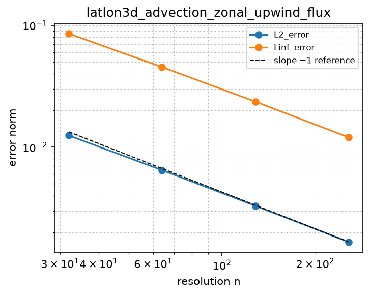
varcoeff_laplacian_lev_noflux_bc
Source: grids/latlon3d/rules/varcoeff_laplacian_lev_noflux_bc.esm
Rewrites ∂(kz·∂u/∂lev)/∂lev at priority 10 — match pattern:
{"op": "D", "args": [{"op": "*", "args": ["kz", {"op": "D", "args": ["u"], "wrt": "lev"}]}], "wrt": "lev"}
where): fires only when u is a bare field shaped [lon, lat, lev]; kz is a bare field shaped [lon, lat, lev]. Under import-edge renaming (§9.7.7) the wrt literal and this shape follow the renamed axis together, so the rule can be imported more than once (each instance scoped to its own grid) without a first-declared-wins collision. A consumer differentiating a compound inline expression must bind it to a declared shaped observed first.Discretization — one makearray tiling the output axes; boundary conditions live in the face regions of this same rule (esm-spec §9.6.8; later regions overwrite earlier, §4.3.2):
| Region | Treatment | Value |
|---|---|---|
lon ∈ [1, NLON], lat ∈ [1, NLAT], lev ∈ [2, NLEV−1] | interior | varcoeff_D_lev_interior(u, kz)[i,j,k] = (varcoeff_lev_face_flux(u[i, j, k], u[i, j, k+1], kz[i, j, k], kz[i, j, k+1], dz[k], dz[k+1]) − varcoeff_lev_face_flux(u[i, j, k−1], u[i, j, k], kz[i, j, k−1], kz[i, j, k], dz[k−1], dz[k])) / dz[k] for i ∈ lon, j ∈ lat, k ∈ [2, NLEV−1] |
lon ∈ [1, NLON], lat ∈ [1, NLAT], lev = 1 | boundary face | varcoeff_D_lev_nf_k1(u, kz)[i,j,k] = varcoeff_lev_face_flux(u[i, j, 1], u[i, j, 2], kz[i, j, 1], kz[i, j, 2], dz[1], dz[2]) / dz[1] for i ∈ lon, j ∈ lat, k ∈ [1, 1] |
lon ∈ [1, NLON], lat ∈ [1, NLAT], lev = NLEV | boundary face | varcoeff_D_lev_nf_kN(u, kz)[i,j,k] = (−varcoeff_lev_face_flux(u[i, j, NLEV−1], u[i, j, NLEV], kz[i, j, NLEV−1], kz[i, j, NLEV], dz[NLEV−1], dz[NLEV])) / dz[NLEV] for i ∈ lon, j ∈ lat, k ∈ [NLEV, NLEV] |
Conservative finite-volume VARIABLE-COEFFICIENT vertical diffusion d/dz(kz du/dz) on the latlon3d non-uniform vertical, with ZERO-FLUX (homogeneous Neumann) walls at BOTH the surface and the model top. This is the vertical turbulent-mixing / boundary-layer (Kzz) operator of a chemical transport model, for a tracer with no surface exchange. Three regions over the full [lon,lat] cross-section: interior k in [2, NLEV-1] (../stencils/varcoeff_D_lev_interior), the surface slab k = 1 (../stencils/varcoeff_D_lev_nf_k1) and the model-top slab k = NLEV (../stencils/varcoeff_D_lev_nf_kN); k = 1 is the ground because the grid’s pe increases with the lev index. Requires NLEV >= 3. EXACT MASS CONSERVATION: every interior face flux is written byte-identically in the two cells that share it, and both wall fluxes are literally absent rather than formed and cancelled, so the column mass sum sum_k dz[k] D[i,j,k] telescopes to exactly 0 in floating point – the operator cannot create or destroy tracer. Reads the free name dz (shape [lev], cell thicknesses; the grid’s lev_thickness applied to the consumer’s pe) and requires kz > 0. Second order (verified 2.00 in L2 and Linf; see tests/conformance/convergence/latlon3d_diffusion_vertical_noflux). For a depositing/emitting tracer use ./varcoeff_laplacian_lev_robin_surface_bc, which shares the interior and model-top slabs and differs ONLY at k = 1. MATCHING. The operator carries a coefficient, so a bare-D match cannot express it; the rule matches the CONSERVATIVE COMPOUND the consumer writes, D( kz * D(u, wrt:lev), wrt:lev ), at priority 10, so under esm-spec 9.6.3 outermost-first compound precedence it fires on the whole compound BEFORE any plain-D rule could lower the inner derivative. That is what lets this diffusion rule COMPOSE in one model with a plain-D vertical ADVECTION rule (e.g. ./ppm_D_lev_mono_noflux_bc, which matches D(f, wrt:lev)): the advective D(c,lev) and the diffusive D(kz*D(c,lev),lev) are structurally distinct patterns and each fires on its own term. Because matching is structural and NON-COMMUTATIVE the consumer MUST write the coefficient on the LEFT: kz * D(u, wrt:lev). A product spelled D(u,lev)*kz, or a compound coefficient expression, does not match (bind a compound coefficient to a declared [lon,lat,lev]-shaped observed first). Mirrors grids/cartesian_uniform_1d/rules/varcoeff_laplacian_zero_flux_bc, lifted to rank 3 on a non-uniform vertical axis.
References
- LeVeque, R. J. (2007). Finite Difference Methods for Ordinary and Partial Differential Equations. SIAM. Section 2.15 (variable-coefficient conservative form) and Section 2.12 (Neumann boundary conditions by dropping the domain-face flux).
- Patankar, S. V. (1980). Numerical Heat Transfer and Fluid Flow. Hemisphere. Chapter 4 (interface conductivity for the conservative control-volume discretisation of a variable-coefficient diffusion flux).
- Jacobson, M. Z. (2005). Fundamentals of Atmospheric Modeling (2nd ed.). Cambridge University Press. Section 8.4 (vertical turbulent diffusion of a tracer) and Section 20.1 (surface emission and dry-deposition flux boundary condition).
Conformance fixtures
- ast:
latlon3d_varcoeff_laplacian_lev_noflux_bc— statusactive - convergence:
latlon3d_diffusion_vertical_noflux— statusactive
Convergence — case latlon3d_diffusion_vertical_noflux
Error norms read from the committed golden tests/conformance/convergence/latlon3d_diffusion_vertical_noflux/golden/errors.json (binding: julia; nothing recomputed for display).
| n | L2_error | observed order | Linf_error | observed order |
|---|---|---|---|---|
| 16 | 8.725e-03 | — | 5.206e-03 | — |
| 32 | 2.178e-03 | 2.00 | 1.325e-03 | 1.97 |
| 64 | 5.442e-04 | 2.00 | 3.338e-04 | 1.99 |
| 128 | 1.360e-04 | 2.00 | 8.373e-05 | 2.00 |
Expected order: 2 (± 0.2).
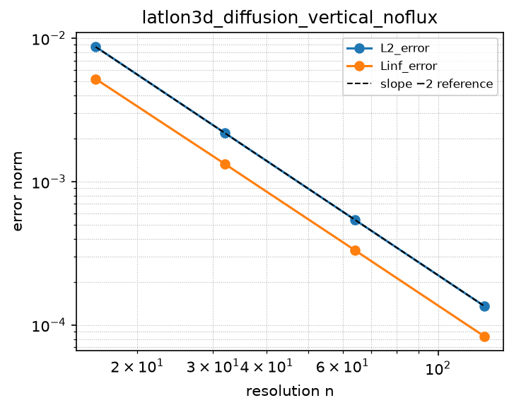
varcoeff_laplacian_lev_robin_surface_bc
Source: grids/latlon3d/rules/varcoeff_laplacian_lev_robin_surface_bc.esm
Rewrites ∂(kz·∂u/∂lev)/∂lev at priority 10 — match pattern:
{"op": "D", "args": [{"op": "*", "args": ["kz", {"op": "D", "args": ["u"], "wrt": "lev"}]}], "wrt": "lev"}
where): fires only when u is a bare field shaped [lon, lat, lev]; kz is a bare field shaped [lon, lat, lev]. Under import-edge renaming (§9.7.7) the wrt literal and this shape follow the renamed axis together, so the rule can be imported more than once (each instance scoped to its own grid) without a first-declared-wins collision. A consumer differentiating a compound inline expression must bind it to a declared shaped observed first.Discretization — one makearray tiling the output axes; boundary conditions live in the face regions of this same rule (esm-spec §9.6.8; later regions overwrite earlier, §4.3.2):
| Region | Treatment | Value |
|---|---|---|
lon ∈ [1, NLON], lat ∈ [1, NLAT], lev ∈ [2, NLEV−1] | interior | varcoeff_D_lev_interior(u, kz)[i,j,k] = (varcoeff_lev_face_flux(u[i, j, k], u[i, j, k+1], kz[i, j, k], kz[i, j, k+1], dz[k], dz[k+1]) − varcoeff_lev_face_flux(u[i, j, k−1], u[i, j, k], kz[i, j, k−1], kz[i, j, k], dz[k−1], dz[k])) / dz[k] for i ∈ lon, j ∈ lat, k ∈ [2, NLEV−1] |
lon ∈ [1, NLON], lat ∈ [1, NLAT], lev = 1 | boundary face | varcoeff_D_lev_robin_k1(u, kz)[i,j,k] = (varcoeff_lev_face_flux(u[i, j, 1], u[i, j, 2], kz[i, j, 1], kz[i, j, 2], dz[1], dz[2]) − (vdep[i, j]·u[i, j, 1] − emis[i, j])·((2·kz[i, j, 1]) / (2·kz[i, j, 1] + vdep[i, j]·dz[1]))) / dz[1] for i ∈ lon, j ∈ lat, k ∈ [1, 1] |
lon ∈ [1, NLON], lat ∈ [1, NLAT], lev = NLEV | boundary face | varcoeff_D_lev_nf_kN(u, kz)[i,j,k] = (−varcoeff_lev_face_flux(u[i, j, NLEV−1], u[i, j, NLEV], kz[i, j, NLEV−1], kz[i, j, NLEV], dz[NLEV−1], dz[NLEV])) / dz[NLEV] for i ∈ lon, j ∈ lat, k ∈ [NLEV, NLEV] |
Conservative finite-volume VARIABLE-COEFFICIENT vertical diffusion d/dz(kz du/dz) on the latlon3d non-uniform vertical, with a ZERO-FLUX model top and a ROBIN SURFACE-EXCHANGE ground – dry deposition out plus prescribed emission in. This is the vertical turbulent-mixing (Kzz / PBL) operator of a chemical transport model coupled to its surface: the operator that carries emitted tracer up out of the bottom layer and delivers depositing tracer back down to it. Identical to ./varcoeff_laplacian_lev_noflux_bc in its interior (../stencils/varcoeff_D_lev_interior, k in [2, NLEV-1]) and its model-top slab (../stencils/varcoeff_D_lev_nf_kN, k = NLEV); the ONLY difference is the surface slab k = 1, which is ../stencils/varcoeff_D_lev_robin_k1 instead of the no-flux one. Requires NLEV >= 3. SURFACE FLUX: the ground flux is closed by RESISTANCE IN SERIES, G_{1/2} = (vdepu[1] - emis) * a/(a + vdep) with a = 2 kz[1]/dz[1] – the half-cell diffusive resistance 1/a and the surface resistance 1/vdep add. Applying vdep directly to the first-cell value instead is INCONSISTENT (an O(1) truncation error that never converges); see ../stencils/varcoeff_D_lev_robin_k1 for the derivation and the measured evidence. Second order in solution error, exactly as the no-flux variant – the surface exchange costs nothing in accuracy (verified 2.00 in L2 and Linf; see tests/conformance/convergence/latlon3d_diffusion_vertical_robin_surface). FREE NAMES: dz (shape [lev], cell thicknesses), plus vdep (deposition velocity, shape [lon,lat], >= 0) and emis (surface emission flux, shape [lon,lat]) read by the surface slab. Requires kz > 0 and 2 kz[i,j,1] + vdep[i,j]dz[1] > 0. MASS: the column budget closes to exactly the physical surface exchange (emis - vdepc_s) per unit area – mass is not conserved, by design; that is the point of the boundary condition. Setting vdep = emis = 0 reproduces ./varcoeff_laplacian_lev_noflux_bc exactly. MATCHING. The operator carries a coefficient, so a bare-D match cannot express it; the rule matches the CONSERVATIVE COMPOUND the consumer writes, D( kz * D(u, wrt:lev), wrt:lev ), at priority 10, so under esm-spec 9.6.3 outermost-first compound precedence it fires on the whole compound BEFORE any plain-D rule could lower the inner derivative. That is what lets this diffusion rule COMPOSE in one model with a plain-D vertical ADVECTION rule (e.g. ./ppm_D_lev_mono_noflux_bc, which matches D(f, wrt:lev)): the advective D(c,lev) and the diffusive D(kzD(c,lev),lev) are structurally distinct patterns and each fires on its own term. Because matching is structural and NON-COMMUTATIVE the consumer MUST write the coefficient on the LEFT: kz * D(u, wrt:lev). A product spelled D(u,lev)*kz, or a compound coefficient expression, does not match (bind a compound coefficient to a declared [lon,lat,lev]-shaped observed first). Mirrors grids/cartesian_uniform_1d/rules/varcoeff_laplacian_zero_flux_bc, lifted to rank 3 on a non-uniform vertical axis.
References
- Wesely, M. L., & Hicks, B. B. (2000). A review of the current status of knowledge on dry deposition. Atmospheric Environment, 34(12-14), 2261-2282. The resistance-in-series surface-exchange formulation.
doi:10.1016/S1352-2310(99)00467-7 - Jacobson, M. Z. (2005). Fundamentals of Atmospheric Modeling (2nd ed.). Cambridge University Press. Section 8.4 (vertical turbulent diffusion of a tracer) and Section 20.1 (surface emission and dry-deposition flux boundary condition).
- LeVeque, R. J. (2007). Finite Difference Methods for Ordinary and Partial Differential Equations. SIAM. Section 2.15 (variable-coefficient conservative form) and Section 2.12 (Neumann boundary conditions by dropping the domain-face flux).
- Patankar, S. V. (1980). Numerical Heat Transfer and Fluid Flow. Hemisphere. Chapter 4 (interface conductivity for the conservative control-volume discretisation of a variable-coefficient diffusion flux).
Conformance fixtures
- ast:
latlon3d_varcoeff_laplacian_lev_robin_surface_bc— statusactive - convergence:
latlon3d_diffusion_vertical_robin_surface— statusactive
Convergence — case latlon3d_diffusion_vertical_robin_surface
Error norms read from the committed golden tests/conformance/convergence/latlon3d_diffusion_vertical_robin_surface/golden/errors.json (binding: julia; nothing recomputed for display).
| n | L2_error | observed order | Linf_error | observed order |
|---|---|---|---|---|
| 16 | 4.896e-03 | — | 6.214e-03 | — |
| 32 | 1.222e-03 | 2.00 | 1.584e-03 | 1.97 |
| 64 | 3.053e-04 | 2.00 | 3.991e-04 | 1.99 |
| 128 | 7.632e-05 | 2.00 | 1.001e-04 | 1.99 |
Expected order: 2 (± 0.2).