divergence_arakawa_c
Stencil
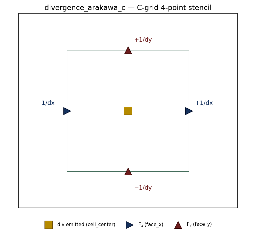
Fx at the two
face_x edges and Fy at the two face_y edges, and emits
div F at the cell center. Stagger metadata is carried in the rule
via requires_locations and emits_location.Coefficients
| selector | stagger | axis | offset | coeff |
|---|---|---|---|---|
arakawa | face_x | $x | 0 | −1 / dx |
arakawa | face_x | $x | +1 | +1 / dx |
arakawa | face_y | $y | 0 | −1 / dy |
arakawa | face_y | $y | +1 | +1 / dy |
The rule declares an arakawa_stagger enum mapping stagger names
(cell_center, face_x, face_y, vertex) to integer codes — the
runtime uses these to dispatch location_centers(grid, ...) per stagger.
requires_locations: ["face_x", "face_y"],
emits_location: "cell_center".
Discrete operator
Let cell \((i, j)\) have center \((x_i, y_j)\) and uniform spacings \(\Delta x, \Delta y\). The flux components live on the staggered C-grid: \(F_x\) at the east/west faces \((x_{i\pm 1/2}, y_j)\) and \(F_y\) at the north/south faces \((x_i, y_{j\pm 1/2})\). With the four faces of cell \((i, j)\) indexed by their stagger offset \(0 / +1\) along the relevant axis, the rule emits the cell-centered divergence
$$\bigl(\nabla \!\cdot\! F\bigr)_{i,j} \;\approx\; \frac{F_x^{\,i+1/2,\,j} - F_x^{\,i-1/2,\,j}}{\Delta x} \;+\; \frac{F_y^{\,i,\,j+1/2} - F_y^{\,i,\,j-1/2}}{\Delta y}.$$Each one-dimensional difference is the centered face-to-center stencil applied to a face-staggered field. Taylor-expanding \(F_x\) about the cell center,
$$F_x^{\,i\pm 1/2,\,j} \;=\; F_x(x_i, y_j) \;\pm\; \tfrac{\Delta x}{2}\,\partial_x F_x \;+\; \tfrac{\Delta x^{2}}{8}\,\partial_x^{2} F_x \;\pm\; \tfrac{\Delta x^{3}}{48}\,\partial_x^{3} F_x \;+\; O(\Delta x^{4}),$$so subtracting the two faces and dividing by \(\Delta x\) cancels the even-order terms exactly:
$$\frac{F_x^{\,i+1/2,\,j} - F_x^{\,i-1/2,\,j}}{\Delta x} \;=\; \partial_x F_x \;+\; \tfrac{\Delta x^{2}}{24}\,\partial_x^{3} F_x \;+\; O(\Delta x^{4}).$$The same expansion in \(y\) gives \(\partial_y F_y + (\Delta y^{2}/24)\,\partial_y^{3} F_y + O(\Delta y^{4})\). Summing the two contributions yields a second-order accurate divergence with a purely dispersive leading error \(\tfrac{\Delta x^{2}}{24}\,\partial_x^{3} F_x + \tfrac{\Delta y^{2}}{24}\,\partial_y^{3} F_y\). Because \(F_x\) and \(F_y\) are sampled at the very faces whose normal flux they represent, no interpolation is needed — the C-grid stagger makes the discrete divergence mimetic with respect to the analytic Gauss identity \(\int_{V_{ij}} \nabla\!\cdot\!F\,dV = \oint_{\partial V_{ij}} F\!\cdot\!\hat{n}\,dS\), and exact for flux fields that are piecewise-linear in each direction.
Convergence
fixtures/convergence/](https://github.com/EarthSciML/EarthSciDiscretizations/blob/main/discretizations/finite_volume/divergence_arakawa_c/fixtures/convergence)
flips from applicable: false to expected_min_order = 2.
The arakawa-staggered manufactured-solution dispatch needed by Layer B
(apply_stencil_2d_arakawa in
EarthSciSerialization.jl/src/mms_evaluator.jl) has landed; the
fixture flip itself is the remaining gate.