ppm_reconstruction
Stencil
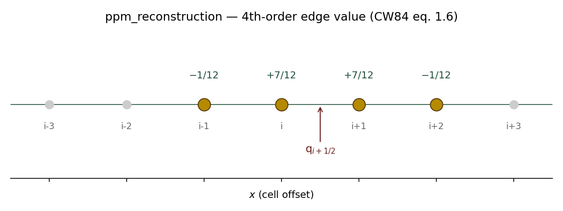
qi+1/2 is a centered combination of cell averages at
offsets −1, 0, +1, +2. Two more cells (−2 and
+2) appear in the rule's broader stencil so the same
edge-value formula applies at qi−1/2.Coefficients
Edge value at q_{i+1/2}:
| selector | offset | coeff |
|---|---|---|
cartesian | −1 | −1/12 |
cartesian | 0 | +7/12 |
cartesian | +1 | +7/12 |
cartesian | +2 | −1/12 |
Per-cell parabola (CW84 eqs. 1.5, 1.7, 1.10):
a_L = q_{i−1/2}(right limit of celli−1)a_R = q_{i+1/2}(left limit of celli+1)da = a_R − a_La₆ = 6·(q_i − ½(a_L + a_R))a(ξ) = a_L + ξ·(da + a₆·(1 − ξ)),ξ ∈ [0, 1]
Limiting (CW84 eqs. 1.10) is not applied at this rule level — see the
flux-limiter rules (flux_limiter_minmod,
flux_limiter_superbee).
Discrete operator
The rule reconstructs a piecewise-parabolic profile inside each cell from cell-averaged inputs \(\bar q_i = \tfrac{1}{\Delta x}\!\int_{x_i-\Delta x/2}^{x_i+\Delta x/2}\!\!q(x)\,dx\) on a uniform Cartesian axis. Reconstruction is two passes — edge values first, parabola coefficients second.
Edge-value pass (CW84 eq. 1.6). A 4-point centered combination of cell averages produces the 4th-order interpolant at \(x_{i+1/2}\):
$$q_{i+1/2} \;=\; \frac{-\,\bar q_{i-1} \;+\; 7\,\bar q_i \;+\; 7\,\bar q_{i+1} \;-\; \bar q_{i+2}}{12}.$$Symmetric Taylor expansion of the four neighbors about \(x_{i+1/2}\) cancels the linear, quadratic, and cubic terms; the leading error is \(-\,\tfrac{\Delta x^{4}}{60}\,q^{(4)}(x_{i+1/2})\), so the edge interpolant itself is fourth-order accurate in the cell average.
Parabola pass (CW84 eqs. 1.5, 1.7). Each cell is represented in a local coordinate \(\xi = (x - x_{i-1/2})/\Delta x \in [0,1]\) by
$$a(\xi) \;=\; a_L \;+\; \xi\,\bigl(\Delta a \;+\; a_6\,(1-\xi)\bigr),$$where \(a_L = q_{i-1/2}\) and \(a_R = q_{i+1/2}\) are the edge values from the first pass and
$$\Delta a \;=\; a_R - a_L, \qquad a_6 \;=\; 6\!\left(\bar q_i - \tfrac{1}{2}(a_L + a_R)\right).$$The choice of \(a_6\) is the cell-mean–conserving constraint \(\tfrac{1}{\Delta x}\!\int a(\xi)\,d\xi = \bar q_i\) — the parabola exactly recovers the cell average regardless of the edge values.
Composing the two passes, point-evaluation at any subcell \(\xi\) recovers \(q(x_{i-1/2} + \xi\,\Delta x)\) with leading error \(O(\Delta x^{3})\) in \(L^\infty\) for smooth profiles. Limiting and discontinuity-detection (CW84 eqs. 1.10, 1.14–1.17) are deliberately omitted at this rule level so the unlimited fourth-order/parabola pair can be exercised in isolation; the flux-limiter rules above compose on top.
Convergence
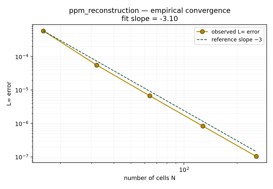
q(x) = sin(2πx) on a periodic
[0, 1] domain, evaluated at subcell coordinates
ξ ∈ {0.1, 0.3, 0.5, 0.7, 0.9}. Empirical slope tracks the
expected −3 reference line.The fixture under
discretizations/finite_volume/ppm_reconstruction/fixtures/convergence/
sets expected_min_order = 2.8 to tolerate pre-asymptotic drift on the
16 → 32 → 64 → 128 sequence; the per-cell sub-sampling settles onto the
third-order asymptote by n = 32.